Phân tích TCO của Nvidia Blackwell Perf – B100 so với B200 so với GB200NVL72
Nvidia’s announcement of the B100, B200, and GB200 has garnered more attention than even iPhone launches, at least among the nerds of the world. The real question that everyone is asking is, what is the real performance increase? Nvidia’s claimed 30x, but is that true? Moreover, the question is really, what is the performance/TCO?
In the last generation, with the H100, the performance/TCO uplift over the A100 was poor due to the huge increase in pricing, with the A100 actually having better TCO than the H100 in inference because of the H100’s anemic memory bandwidth gains and massive price increase from the A100’s trough pricing in Q3 of 2022. This didn’t matter much though because the massive requirements in the AI industry for training as opposed to inference benefited more from H100’s greater FLOPS performance, and most the price increase was driven by opportunistically high margins from Nvidia.
With Blackwell, that all changes as pricing is not up nearly as much generationally. This is due to competition from existing huge volumes of H100s and H200s and emerging challengers such as hyperscale custom silicon, AMD’s MI300X and Intel’s Gaudi 2/3 entering the market and making their own performance/TCO arguments. As such, Nvidia must make a compelling argument to sell their new generation. Of course, they aren’t letting competition encroach in, with very aggressive, perhaps even benevolent pricing.
Nvidia has claimed as much as 30x higher performance for Blackwell over Hopper. The problem is that the 30x figure is based on a very specific best-case scenario. To be clear, this scenario is certainly realistic and possible to achieve (outside of unfair quantization differences) but is not exactly a scenario that is representative of the market. Today, let’s walk through Nvidia’s performance claims, and home in on the actual performance uplift for a variety of applications including inference and training on a variety of model sizes using the LLM model performance simulator that we have been building for over the last 1.5 years. We will also dissect whether the competition has a shot when selling their merchant silicon and if hyperscale silicon is competitive with Nvidia’s new offerings despite a massive cost difference.
There are a handful of primary workloads that should be tracked, and each has varying characteristics. Inference versus training is quite different obviously due to the backwards pass in training and difference in batch sizes. Working with large size models can lead to very different performance characteristics as well as one breaks GPU and node boundaries – for instance extending parallelism beyond the 8 GPUs in a typical HGX H100 server.
Many folks tend to focus in on small model inference today (<100 billion parameters) when discussing performance, but with Blackwell pushing the cost of inference down so dramatically, and with workload needs continuing to be met poorly by small models, combined with the release of open models such Databricks DBRX 132B, xAI Grok-1 314B Cohere Command R+ 104B, Mistral 8x22B, as well as the upcoming Meta LLAMA 3 release, it is clear that the focus will shift back towards inference performance for large models.
Larger than 100 billion parameter models will be the new norm for “small model” fine tuning and inference, and larger than 1 trillion parameter sparse models will be the norm among large models. To be clear, these large models already take up most of the inference and training compute today. The bar for large models will only continue to move higher with future model releases. Remember that to make economic sense, hardware has to stick around and be effective for 4-6 years, not just until the next model release.
Let’s start off by looking at specifications before diving into our LLM performance simulator and what it tells us about large and small model inference versus training.
The performance gains showcased at the keynote speech were achieved through improvements across multiple dimensions – with the foundation and easiest to understand factor being simply the improvements in memory bandwidth and floating-point operation (FLOPS) capacity.
The air-cooled 700W B100 will be the first to ship and will deliver 1,750 TFLOPS of FP16/BF16 compute. The B100’s baseboard is made to slot into the same design used in today’s HGX H100 systems – forcing the B100 to run at lower power and clock speeds to remain within the thermal envelope of existing systems. Very soon after the B100 ships, the B200 will come to market at a higher power and faster clock speed, delivering 2,250 TFLOPS of FP16/BF16 compute. Furthermore, the use of liquid cooling in the GB200 NVL72 will allow the Blackwell GPU to run at even higher power levels, unlocking further performance upside – delivering 2,500 TFLOPS of FP16/BF16 compute – a 153% improvement over the H100 and H200. There is also a 1200W B200 that is not included in the table.
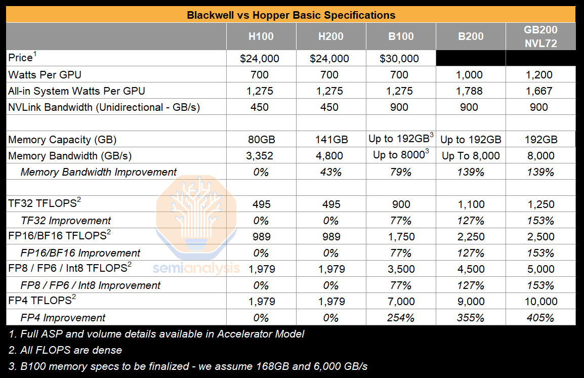
FLOPS are only up 77% on FP16 and TF32 with B100, but as power increases, and combining further quantization, total FLOPS can scale to as much as 4x. Memory Bandwidth, arguably the most important specification upgrade, grows from 3.4 TB/s in the H100 and 4.8 TB/s in the H200 to up to 8.0 TB/s in the Blackwell family – this most directly improves inference throughput and interactivity (tokens/second/user) because inference is often memory bandwidth constrained.
We should note that, even in the worst-case scenario, FP16 vs FP16, FLOPS are up 153% gen on gen, but memory bandwidth gains are smaller. The bandwidth gains from A100 to H100 were larger than that of this generation. The memory wall is one of the greatest challenges facing the AI industry for future scaling.

More important is to look at FLOPS times number of bits divided by bandwidth; this metric shows the real story. At most number formats, the ratio is about the same, i.e. the arithmetic intensity required to fully utilize the FLOPS stays stable. Putting aside the advent of a new number format, most code should port and achieve similar utilization given the arithmetic intensity. Once all the new tricks of the Blackwell tensor core are fully utilized though, there should be better MFU on Blackwell versus Hopper generally.
However – these performance gains should be viewed in the context of the fact that the silicon area of Blackwell (~1600mm2 with 208B transistors) is double that of Hopper (~800mm2 with 80B transistors). Nvidia, given the slowdown of Moore’s law and 3nm issues, had to deliver generational performance without a real process node shrink. Through the use of DTCO and a mild 6% optical process shrink Blackwell was still able to deliver twice the performance of Hopper.
When looking at raw TFLOPS/mm2 of silicon, i.e. benching against logic manufacturing cost, the B100 actually delivers less performance, a 77% improvement in FLOPS, versus a ~100% growth in silicon area. This is due to the underclocking to hit the existing 700W platforms for quick time to market, and it is only in the B200 and GB200 NVL72 where we see per silicon area improvements.
Normalizing by silicon area gain, the air-cooled B200 only delivers a 14% FP16 FLOPS improvement per silicon area – hardly what one would expect from a brand-new architecture. Because most of the performance gain was simply through more silicon area and quantization. People need to understand how microscaling works and solve FP8, FP6, and FP4 training with the Blackwell architecture.

Also note throughout this piece we show FP4 and FP6 FLOPS for H100 and H200 as the same as FP8 FLOPS. While there is a slight overhead casting up the format to FP8 after loading from memory as FP4, in compute bound scenarios, the memory bandwidth savings reduce power consumption enough and give more headroom for achieving max FLOPS, which effectively wipes away overhead in real world use cases.
Given the premise that twice the silicon area should require twice the power, it is important to analyze the isopower performance gains – that is – the FLOPS achieved per GPU watt.

While the B100 does deliver 77% more FLOPS of FP16/BF16 with the same 700W of power, the B200 and GB200 both deliver diminishing improvement in FLOPS for every incremental power delivered to the chip. The GB200’s 47% improvement in TFLOPS per GPU Watt vs the H100 is helpful – but again hardly anything to write home about without further quantization of models, and as such is certainly not enough to deliver the 30x inference performance showcased in the keynote address.
The FLOPS cost similarly is unremarkable. The TFLOPS per $ for the GB200 NVL and B200 are not a meaningfully different story.

As the above simple analysis makes clear, specs alone are only a small part of the story and the vast majority of the claimed 30x inference performance gains are from quantization as well as architectural improvements along other game changing dimensions.
Nvidia claims 30x performance gains with GB200 versus H200, but as the above analysis demonstrates, no single specification comes anywhere close to that uplift.
How is that possible? Well, it’s because systems matter more than just individual chip specifications. FabricatedKnowledge had a fantastic think piece on the Jensen’s “Datacenter is the unit of compute” line that he’s been saying for years but has finally come to fruition with the GB200 NVL72. We should note that the NVLink backplane and rack level product is not new in the context of machine learning hardware.
Google has been shipping 64 TPU passive copper connected subslices that are optically connected beyond that with fully water-cooled racks since 2018. The major distinction between TPUv5p (Viperfish) and TPUv5e (Viperlite) besides chip level specs is that the v5e (Viperlite) connects 256 TPUs with copper while not scaling out further and the v5p (Viperfish) connects 64 with copper and connects to the rest of the pod of 8960 through the Optical Circuit Switch (OCS).

Below is probably the coolest chart we’ve ever seen regarding machine learning performance modeling and the search space of optimal total cost of ownership (TCO). It reveals a lot about LLM performance modeling and trends. It also shows a variety of different parallelism strategies, batch sizes.

When running inference on smaller models on a single GPU, you generally end up with a curve like the below which shows very high interactivity (tokens/second/user) at low batch sizes, and as you increase batch size, throughput grows, but interactivity also comes down. There is a tradeoff curve between system throughput for all users (cost per token) versus single user interactivity (user experience).

Unfortunately, the simplicity of a single tradeoff curve is wiped away with massive models such as GPT-4. Massive models must be split amoung many GPUs, which introduces many complications.

For example, with GPT-4 MoE’s 55B attention parameters and 16 experts of 111B parameters each across 120 layers, that’s 1.831 trillion parameters at 8 bits per parameter, in total requiring 1,831 GB of memory.

It is impossible for this model to fit on a single GPU or even an 8 GPU server. As such, it must be split across dozens of GPUs. How the model is split is very important as each different configuration means very different performance characteristics.
Let’s start simple and work our way up.
Parallelism, splitting tasks across multiple GPUs, is necessary just to fit the model into a system. But as we will see – parallelism can do much more than just alleviate this capacity constraint. Let’s explain the most important forms of parallelism and how the use of varying configurations of parallelism is at the core of the performance gains. We will start with a simplified explanation which overlooks some complexity to make it more approachable before going into the real model which does account for KVCache, prefill, and various memory, compute, and communication overhead.
In pipeline parallelism, the simplest form of parallelism, the model’s layers are split up across multiple GPUs – in the example below using GPT-4 MoE, splitting the 120 layers across 16 GPUs.
Each token in each user’s query is sent sequentially through each GPU during the forward pass across all layers until it runs through the entire model. Because there are fewer layers per GPU, the model can now be held across all 16 GPUs.

However – since the tokens in the query still have to pass sequentially through all the GPUs in the pipeline parallelism setup – there is no net improvement in interactivity (tokens/second/user).
Comparing the PP16 setup above to a hypothetical one GPU deployment, we see that the interactivity is the same (ignoring the FLOPS and memory capacity constraint of the 1 GPU system – which is triggered in the case of inference on GPT-4 MoE with 100 users).
The main benefit of pipeline parallelism is that memory capacity pressures are alleviated – making the model fit, and not about making it fast. Each stage of the pipeline would work on a seperate set of users sequentially.
Both Pipeline Parallelism and Tensor Parallelism have the benefit of overcoming memory capacity constraints (i.e. fitting the model into the system), but in tensor parallelism, every layer has its work distributed across multiple GPUs generally across the hidden dimension. Intermediate work is exchanged via all-reductions across devices multiple times across self-attention, feed forward network, and layer normalizations for each layer. This requires high bandwidth and especially needs very low latency.
In effect, every GPU in the domain works together on every layer with every other GPU as if there were all one giant GPU. The below diagram demonstrates the two networks within a DGX H100 – namely the NVLink Scale up network (multicolored lanes connecting to the NVSwitch) and the InfiniBand/Ethernet scale-out network accessed via the ConnectX-7 network interface cards in orange.
Scale up networks like NVLink and Google’s ICI enable tensor parallelism to be much faster than scale out networks.

Tensor Parallelism allows memory bandwidth to be pooled and shared across all GPUs. This means that instead of only 8,000 GB/s of memory bandwidth available to load model parameters for each layer during the forward pass, 128,000 GB/s is now available.
In the below example, interactivity (tokens/second/user) is 16 times better than the PP16 example, at 69.9 tokens/second/user vs the 4.4 achieved in the PP16 system. Total system throughput is accordingly 16 times greater as well, in this simplistic example.

The example presented above, however, is the perfect scenario, without taking into account various factors that lead to the lower memory bandwidth utilization (MBU) that are observed in reality. The most important effect to note here is the communications penalty created by the need for all-reduce and all-to-all operations among GPUs. The greater the number of GPUs in the tensor parallelism, the more this effect acts to diminish interactivity and throughput.
In reality, pipeline parallelism achieves higher throughput than tensor parallelism due to less GPU-to-GPU communication bottlenecks. It also generally achieve higher batch sizes / MFU.
While in Tensor Parallelism, all of the GPUs work together to host all layers, in Expert Parallelism, the experts are split amongst different GPUs, but attention is replicated.
In the below example of an EP16 system, each GPU hosts one expert. This lowers the total parameters loaded to only 166 B per expert domain, that is 55B for the replicated attention and 111B for each expert.

The fact that each expert domain also has to load the attention imposes additional overhead in the form of memory bandwidth requirements per token. Thus, with greater memory bandwidth needs in EP vs TP, the ratio of memory bandwidth available to bandwidth required to load the model is lower for the EP16 example vs the TP16 example, resulting in lower interactivity of 48.2 for EP16 vs 69.9 for TP16, and commensurately lower throughput.
Recall that the use of Tensor Parallelism imposes a major communications penalty on memory bandwidth utilization, slowing down throughput. This effect is in opposition to the additional overhead from the attention layer in expert parallelism – and the degree of this communications penalty determines which effect dominates.
Expert parallelism also has communication overhead as shown by the graphic above, but splitting expert domains and replicating attention means significantly less overhead. Basically, the All Reduce and All to All operations on the right side of the graphic do not need to be executed in expert parallelism. We should also note parallel transformers have a huge improvement in inference and training costs, especially as model sizes scale, precisely due to requiring less communication within each layer. There are challenges implementing them at scale though, at least in the open model world.
Data parallelism is perhaps the simplest of all the parallelisms – essentially it replicates everything about the system without sharing or consolidating any system resources. It’s like having a web server in the US and Asia. Different users are hitting each server and they are running the same stuff, but completely independent of each other.
In the example below, there is no interactivity speed up because each Data Parallel System of TP16 has already hit the memory wall. Keeping the same number of total users at 100, total throughput is also the same as in the TP16 example. Data parallelism increases the headroom at which you can increase the number of users before hitting the FLOPS constraint due to having 32 total GPUs worth of FLOPS available (vs 16 for TP16), but if we do not introduce more users to the system, hence generating more throughput, going from TP16 to TP16 DP2 is a waste of resources.

If we were to keep the 100 users on our prior TP16 system example but implement two data parallel systems – that is 200 users in total, then we would have twice the throughput. The most important benefit of data parallelism is that there is no overhead given each data parallel system operates completely independently. We should note that while for the other systems we handwaved away all the overheads for sake of simplicity in the explanation, with data parallel, there aren’t any overheads!
We can stack up the various parallelism schemes as well to suit a given set of models, users, and interactivity as well as throughput objectives.
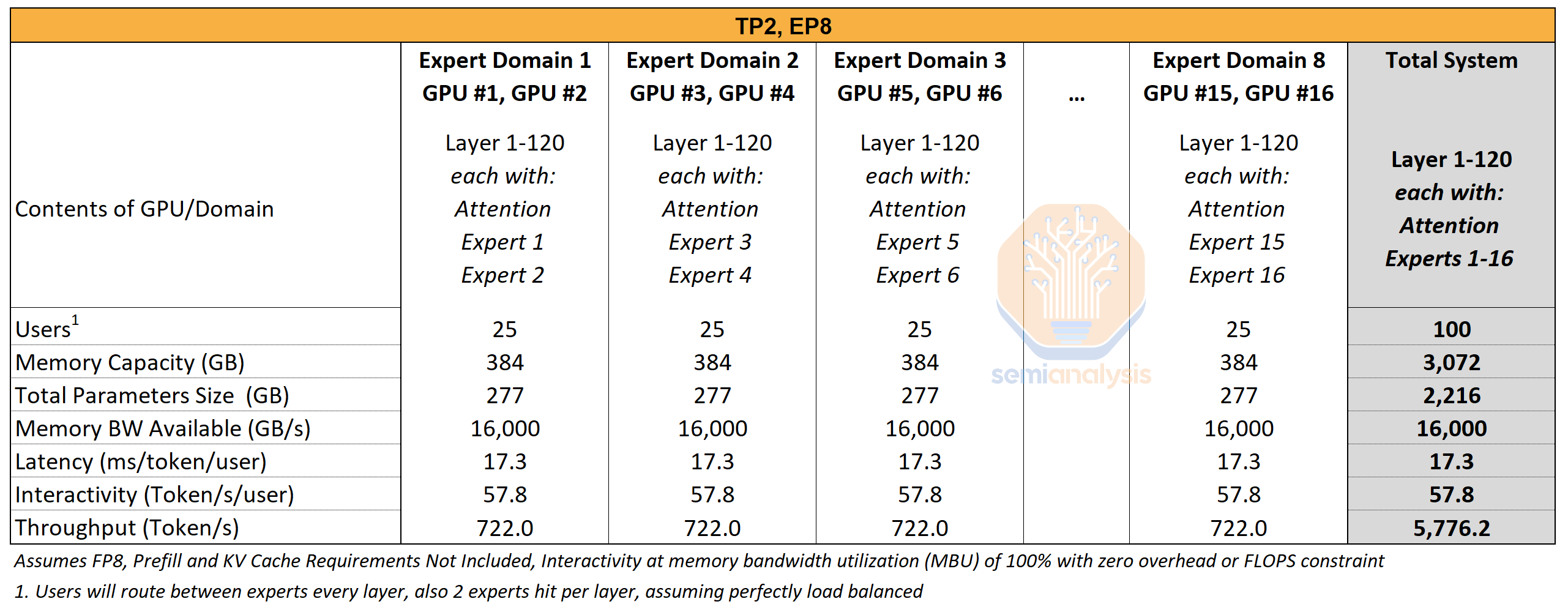
In the below example of TP2 EP8 Parallelism, we implement 8 expert domains, with two GPUs in each domain operating in TP2 Tensor Parallelism. Compared to EP16 Parallelism, each expert domain now loads two experts’ worth of parameters plus attention as opposed to one expert parameters plus attention – thus reducing memory capacity needed overall and bandwidth overhead. The total system parameters memory requirement is therefore lower at 2,216 GB in TP2 EP8 vs EP16 with 2,656 GB of memory requirements.
This enables higher interactivity at 57.8 tokens/s/user in TP2 EP8 vs 48.2 tokens/s/user in EP16. However, while there is less memory capacity/bandwidth overhead – moving to TP2 EP8 will introduce a communications penalty which again is omitted from this analysis.
The unveiling of the GB200 NVL72 made waves – partially for the wrong reasons – and led to quite a bit of salivation over increased liquid cooling content and much higher data center power density. NVL72 enabled a non-blocking all to all network among 72 GPUs running at 900 GB/s unidirectional bandwidth, far faster than the 50 GB/s (400G) currently delivered by InfiniBand/Ethernet scale out networks. More importantly than the bandwidth increases, the NVL72 also attains lower latency.
Putting everything together – the main innovation of NVL72 is that it vastly expands the set of parallelisms that are enabled by the NVLink network. The H100 and H200’s 8 GPU NVLink network only allowed a small set of configurations – for instance, the list of practical permutations of Tensor Parallelism and Expert Parallelism is not long: (TP1 EP8), (TP2 EP4), (TP4 EP2) and (TP8, EP1). We say practical because you can run tensor parallelism outside of a single server, but doing this murders your performance.
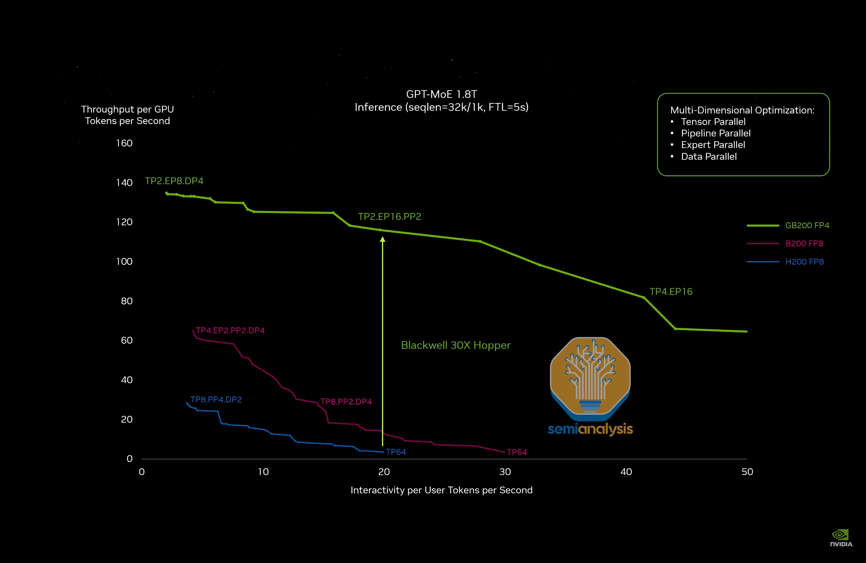
When looking at the H200 running GPT-4 at FP8, the pareto optimal frontier of parallelism options cliffs off quite badly as the number of GPUs employed for tensor parallelism grows.
At TP8, the GPUs are all communicating via NVLink, and so the penalties aren’t that bad as interactivity (tokens per second per user) is scaled higher, but then, all of a sudden, the throughput tanks. This is due to TP being extended beyond 8 GPUs. To go from interactivity of ~6.3 to ~6.5 drives a ~23% decrease in total throughput per GPU. This is a very gnarly impact that is all because communications for tensor parallelism must now cross the boundary out of the NVLink network and onto InfiniBand/Ethernet.

The primary cause of this is because the latency to get from one GPU to another is relatively high when going through a ConnectX-7 NIC in addition to a network switch. Furthermore, there are often DSPs and Optics involved, or AECs to pass through to cross server to server. In contrast, NVLink networks only require passing through the NVLink Switch, and otherwise purely short reach copper.
Furthermore, this impact occurs yet again when hitting >16 and >32 GPUs for tensor parallelism.
With this in mind – turning to the slide from the keynote speech – notice that the slide Nvidia used has chosen to benchmark off of TP64, the worst possible parallelism scheme to run on the H200.

Not only that, but Nvidia also intentionally handicapped the H200 and B200 systems with FP8 despite using FP4 on the GB200. All of these systems could benefit from a memory perspective with using FP4, which would push all of these curves to the right with regards to the interactivity metric. Furthermore, B200 was limited to FP8 despite also having 2x the FLOPs at FP4.
The most obvious factor explaining the 30x performance gain is comparing GB200 NVL performance at FP4 vs the H200 and B200 using FP8 quantization. Peeling this in our simulator shows we have only an ~18x performance gain from the H200 to the GB200. Not nearly as shocking as Nvidia made it out to be with 30x gains, but still an incredibly impressive feat.
The next most impactful factor is somewhat more subtle – the benchmark scenario which imposes a 32k input, 1k output for GPT-4 with a 5 second time to first token (TTFT) generation constraint on all benchmarks. Prefill is extremely FLOPS bound, and as such any limitations here are very hard on lower FLOPS systems like the H200. Furthermore, by maxing out the prefill tokens per user, and minimizing decode, these constraints get even tighter.
This scenario games the benchmark by effectively eliminating all large batch size system setups using an H200 system, as running a large batch size on an H200 system would blow way past the 5 seconds time to first token constraint due the lower FLOPS. Without large batch sizes, there is no way the H200 system can deliver high overall system throughput – meaning the H200 curves are lower than they otherwise would be if not for the 5 second constraint.
To be clear, it is very desirable to have lower time to first token, but that is a tradeoff for the user to consider and make. This benchmark diminishes the performance envelope in terms of throughput that could be achieved by an H200 system albeit at some tradeoff against time to first token.
If this was a 512 input 2k output scenario, with the same 5 second time to first token (TTFT) and 20 interactivity requirements, performance gains are less than 8x. We aren’t sure of at scale deployment ratios of input vs output tokens though, and it’s possible many people require extremely high input and low output ratios. Potentially agent and other emerging workloads will have even higher ratios of prefill to decode than the 32:1 ratio that Nvidia presented.
The performance gains are still remarkable in this cherry-picked scenario due to architectural and networking gains, even after peeling away the impact of pure specs and marketing gimmicks.
Now instead let’s look at real performance and TCO improvements across what we consider more realistic scenarios of various model sizes and training versus inference. Furthermore, lets dive into what these performance gains drive for profitability of inference systems.
When we run our model simulator, we get very different performance uplift per GPU SKU. Next let’s dive into the performance and TCO improvements across from H100/H200 to B100, B200, and GB200 large models and small models in both training and inference. Furthermore, we will show figures for revenue, cost, and profitability per inference system for GPT-4 at scale.