Lượng tử hóa mạng nơ-ron và định dạng số từ những nguyên tắc đầu tiên

Quantization has played an enormous role in speeding up neural networks – from 32 bits to 16 bits to 8 bits and soon further. It’s so important that Google is currently being sued for $1.6 billion to $5.2 billion for allegedly infringing on BF16 by its creator. All eyes are on number formats as they are responsible for a massive chunk of AI hardware efficiency improvements in the past decade. Lower precision number formats have helped push back the memory wall for multi-billion-parameter models.

Nvidia, for one, claims that it is the single largest component of the 1000x improvement in single-chip TOPS in the past 10 years, adding up to 16x. For comparison, the improvement in process technology from 28nm to 5nm has only been 2.5x!

In this article we’ll do a technical dive from the very basic fundamentals of number formats to the current state of the art on neural network quantization from a first principles basis. We will cover floating point versus integer, circuit design considerations, block floating point, MSFP, Microscaling Formats, log number systems, and more. We will also cover the differences in quantization and number formats for inference and high precision vs low precision training recipes.

Furthermore, we will discuss what’s next from models given challenges with quantizing and accuracy losses associated. Lastly, we will cover the hardware developers such as Nvidia, AMD, Intel, Google, Microsoft, Meta, Arm, Qualcomm, MatX and Lemurian Labs will be implementing as they scale past the currently popular 8 bit formats such as FP8 and Int8.

The bulk of any modern ML model is matrix multiplication. In a GPT-3, massive matrix multiplications are used in every layer: for example, one of the specific operations is a (2048 x 12288) matrix multiplied by a (12288 x 49152) matrix, which outputs a (2048 x 49152) matrix.

What’s important is how each individual element in the output matrix is computed, which boils down to a dot product of two very large vectors – in the above example, of size 12288. This consists of 12288 multiplications and 12277 additions, which accumulate into a single number – a single element of the output matrix.

Typically, this is done in hardware by initializing an accumulator register to zero, then repeatedly

all with a throughput of 1 per cycle. After ~12288 cycles, the accumulation of a single element of the output matrix is complete. This “fused multiply-add” operation (FMA) is the fundamental unit of computation for machine learning: with many thousands of FMA units on the chip strategically arranged to reuse data efficiently, many elements of the output matrix can be calculated in parallel to reduce the number of cycles required.

All numbers in the diagram above need to be represented in some way in bits somewhere inside the chip:

• x_i, the input activations

• w_i, the weights

• p_i, the pairwise products

• All intermediate partially-accumulated sums before the entire output is finished accumulating

• The final output sum

Out of this large design space, most of ML quantization research these days boils down to two goals:

1. Achieving good energy and area efficiency. This is primarily dependent on the number formats used for the weights and for the activations.

2. Storing the hundreds of billions of weights accurately enough, while using as few bits as possible to reduce the memory footprint from both capacity and bandwidth standpoint. This is dependent on the number format used to store the weights.

These goals are sometimes aligned and sometimes at odds – we’ll dive into both.

The fundamental limit to compute performance in many ML chips is power. While the H100 can on paper achieve 2,000 TFLOPS of compute, it runs into power limits before then – so the FLOPs per joule of energy is an extremely relevant metric to track. Given that modern training runs now regularly exceed 1e25 flops, we need extremely efficient chips sucking megawatts of power for months in order to beat that SOTA.

First, though, let’s dive into the most basic number format in computing: the integer.

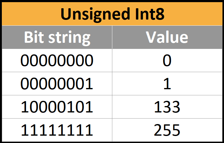
Positive integers have the obvious base-2 representation. These are called UINT, for unsigned integer. Here are some examples of 8-bit unsigned integers, otherwise known as UINT8, which goes from 0 to 255.

There can be any number of bits in these integers, but usually only these four formats are supported: UINT8, UINT16, UINT32, and UINT64.

Negative integers need a sign to distinguish between positive and negative. We can just put an indicator in the most significant bit: e.g. 0011 means +3, and 1011 is –3. This is called sign-magnitude representation. Here are some examples of INT8, which goes from –128 to 127. Note that because the first bit is a sign, the maximum has effectively halved from 255 to 127.

Sign-magnitude is intuitive but inefficient – your circuitry has to implement pretty significantly different addition and subtraction algorithms, which are in turn different from the circuitry for unsigned integers without the sign bit. Interestingly, hardware designers can get around this problem by using two’s complement representation, which enables using the exact same carry-adder circuitry for positive, negative, and unsigned numbers. All modern CPUs use two’s complement.

In unsigned int8, the maximum number 255 is 11111111. If the number 1 is added, 255 overflows to 00000000, IE 0. In signed int8 the minimum number is -128 and maximum is 127. As a trick to have INT8 and UINT8 share hardware resources, -1 can be represented by 11111111. Now when the number 1 is added, it overflows to 00000000, representing 0 as intended. Likewise, 11111110 can be represented as -2.

Overflows are used as a feature! Effectively, 0 through 127 are mapped as normal and 128 through 255 are directly mapped to -128 to -1.

To take this 1 step further, we can make a new number format with ease on existing hardware without modifications. While these are all integers, you can just as trivially imagine that they’re multiples of something else! For example, 0.025 is just 25 thousandths, and it can just be stored as the integer 25. Now we just need to remember somewhere else that all the numbers being used are in thousandths.

Your new “number format” can represent numbers in thousandths from –0.128 to 0.127, with no actual logic changes. The full number is still treated as an integer and then the decimal point is fixed in the third position from the right. This strategy is called fixed point.

More generally, this is a helpful strategy that we’ll revisit a lot in this article – if you want to change the range of numbers that you can represent, add a scale factor somewhere. (Obviously, you’d do this in binary, but decimal is easier to talk about)

Fixed point has some disadvantages though, particularly for multiplication. Let’s say you need to calculate one trillion times one trillionth – the huge difference in size is an example of high *dynamic range*. Then both 10¹² and 10^-12 must be represented by our number format, so it’s easy to calculate how many bits you need: count from 0 to 1 trillion in increments of one trillionth, you need 10^24 increments, log2(10^24) ~= 80 bits to represent the dynamic range with the level of precision we would like.

80 bits for every single number is pretty wasteful in obvious ways. You don’t necessarily care about the absolute precision, you care about the relative precision. So even though the above format is able to distinguish between exactly 1 trillion and 999,999,999,999.999999999999, you generally don’t need to. Most of the time, you’re instead concerned with the amount of error relative to the size of the number.

This is exactly what scientific notation addresses: in our previous example, we can write one trillion as 1.00 * 10^12 and one trillionth as 1.00 * 10^-12, which is much less storage. This is more complex but lets you represent extremely large and small numbers in the same contexts with no worries.

So in addition to the sign and value, we now have an exponent as well. IEEE 754-1985 standardized the industry-wide way to store this in binary, out of the many slightly different formats being used at the time. The main interesting format, the 32-bit floating point number (“float32” or “FP32”) can be described as (1,8,23): 1 sign bit, 8 exponent bits, and 23 mantissa bits.

• The sign bit is 0 for positive, 1 for negative.

• The exponent bits are interpreted as an unsigned integer, e, and represent the scale factor 2^e-127, which can take on a value somewhere between 2^-126 and 2¹²⁷. More exponent bits would mean more dynamic range.

• The mantissa bits represent the value 1.<mantissa bits>. More mantissa bits means more relative precision.

This is somewhat simplified – some special cases (subnormals, infinities, and nans) exist but are a story for another time. Just know that floating point is complicated and has special cases that need to be handled separately by the hardware.

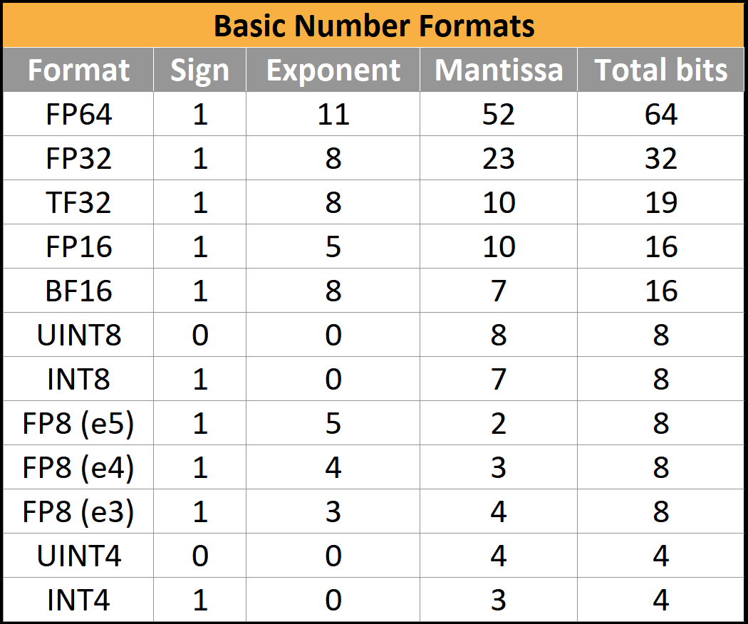
Other bit widths have been standardized or de facto adopted, for example FP16 (1,5,10), and BF16 (1,8,7). There the argument is centered around range versus precision.

FP8(1,5,2 or 1,4,3) has some additional quirks recently standardized in an OCP standard, but the jury is still out. Many AI hardware firms have implemented silicon with slightly-superior variants which are incompatible with the standards.

Coming back to hardware efficiencies, the number format used has a tremendous impact on the silicon area and power required.

Integer adders are some of the best-studied silicon design problems of all time. While the real implementations are substantially more complex, one way to think of adders is to imagine them as adding and carrying the 1 as needed all the way up the sum, so in some sense an n-bit adder is doing an amount of work proportional to n.

For multiplication, think back to grade school long multiplication. We do an n-digit times 1-digit product, then adding up all the results at the end. In binary, multiplying by a 1-digit number is trivial (0 or 1). This means the n-bit multiplier essentially consists of n repetitions of an n-bit adder, so the amount of work is proportional to n^2.

While real implementations are vastly different depending on area, power, and frequency constraints, generally 1) multipliers are far more expensive than adders, but 2) at low bit counts (8 bits and below) the power and area cost of an FMA has more and more relative contribution from the adder (n vs n^2 scaling)

Floating point units are substantially different. In contrast, a product/multiplication is relatively simple.

• The sign is negative if exactly one of the input signs is negative, otherwise positive.

• The exponent is the integer sum of the incoming exponents.

• The mantissa is the integer product of the incoming mantissas.

A sum in contrast quite complex.

• First, take the difference in exponents. (Let’s say exp1 is at least as large as exp2 – exchange them in the instructions if not)

• Shift mantissa2 downward by (exp1 – exp2) so that it aligns with mantissa1.

• Add in an implicit leading 1 to each mantissa. If one sign is negative, perform a two’s complement of one of the mantissas.

• Add the mantissas together to form the output mantissa.

• If there is an overflow, increase the result exponent by 1 and shift the mantissa downward.

• If the result is negative, convert it back to an unsigned mantissa and set the output sign to be negative.

• Normalize the mantissa so that it has the leading 1, and then remove implicit leading 1.

• Round the mantissa appropriately (usually round-to-nearest-even).

Remarkably, floating point multiplication can even cost *less* than integer multiplication because there are fewer bits in the mantissa product, while the adder for the exponent is so much smaller than the multiplier that it almost doesn’t matter.

Obviously, this is also extremely simplified, and in particular, denormal and nan handling which we haven’t gone into takes up a lot of area. But the takeaway is that in low bit count floating point, products are cheap while accumulation is expensive.

All pieces we mentioned are quite visible here – adding up the exponent, a large multiplier array for the mantissas, shifting and aligning things as needed, then normalizing. (Technically, a true “fused” multiply-add is a bit different, but we omit that here.)

This chart illustrates all of the above points. There is a lot to digest, but the main point is that accumulation of INT8 x INT8 with accumulation into fixed point (FX) is the cheapest and is dominated by the multiplication (“mpy”), whereas using floating point for either operand or accumulation formats are (often hugely) dominated by the cost of the accumulation (“alignadd” + “normacc”). For example, a lot of savings are possible by using FP8 operands with a *fixed point* accumulator rather than the usual FP32.

All in all, this and other papers claim that an FP8 FMA will take 40-50% more silicon area than an INT8 FMA, and energy usage is similarly higher or worse. This is a large part of why most dedicated ML inference chips use INT8.

Since integer is always cheaper, why don’t we use INT8 and INT16 everywhere instead of FP8 and FP16? It comes down to how accurately these formats can represent the numbers that actually show up in neural networks.

We can think about every number format as a lookup table. For example, a really dumb 2-bit number format might look like this:

Obviously, this set of four numbers isn’t terribly useful for anything because it’s missing so many numbers – in fact, there are no negative numbers at all. If a number in your neural network doesn’t exist in the table, then you all you can do is round it to the nearest entry, which introduces a little bit of error into the neural network.

So what is the ideal set of values to have in the table, and how small of a table can you get away with?

For example, if most of the values in a neural network are near zero (which they are in practice) we would like to be able to have a lot of these numbers near zero, so we can get more accuracy where it matters by sacrificing accuracy where it doesn’t.

In practice, neural networks are typically normal or laplace distributed, sometimes with substantial outliers depending on the exact numerics of the model architecture. In particular, with extremely large language models, extreme outliers tend to emerge that are rare but important to the functionality of the model.

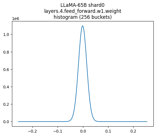
Above shows the weights of part of LLAMA 65B. This looks quite like a normal distribution. If you compare this with the distributions of numbers in FP8 and INT8, it’s pretty obvious that floating point focuses where it matters – near zero. This is why we use it!

It’s still not a great match to the real distribution, though – it’s a bit too pointy still with sharp cutoffs every time the exponent increments, but way better than int8.

Can we do better? One way to design a format from scratch is to minimize the mean absolute error – the average amount you are losing from rounding.

For example, Nvidia at HotChips touted a Log Number System as a possible path forward to continue scaling past 8 bit number formats. The error from rounding is generally smaller with a log number system, but there are a number of problems including the incredibly expensive adders.

NF4 and variants (AF4) are 4-bit formats that use an exact lookup table to minimize the error assuming weights follow a perfectly normal distribution. But this approach is extremely expensive in area and power – every operation now requires a lookup into a huge table of entries, which is far worse than any INT/FP operation.

A number of alternative formats exist: posits, ELMA, PAL, and others. These claim various benefits on compute efficiency or representational accuracy, but none of them have yet reached commercially relevant scale. Perhaps one of these, or one yet to be published/discovered, will have the cost of INT with the representational accuracy of FP – several already make that claim, or better.

We personally are most hopeful for Lemurian Labs PAL, but there is a lot that has not yet been disclosed regarding their number formats. They claim their accuracy and range is better at 16 bits than both FP16 and BF16, while also being cheaper in hardware.

As we continue to scale past 8-bit formats, PAL4 also claims a better distribution than log number systems like Nvidia floated at HotChips. Their on-paper claims are amazing, but there is no hardware that has implemented the format… yet.

One interesting observation is that elements are almost always similar in magnitude to nearby elements in the tensor. And when elements of a tensor are much larger than usual, nearby elements essentially don’t matter – they’re comparatively too small to be seen in the dot product.

We can take advantage of this – instead of having a floating point exponent on every number, we can share one exponent between several elements. This saves a lot of mostly-redundant exponents.

This approach has been around for a while – Nervana Flexpoint, Microsoft MSFP12, Nvidia VSQ – and just in 2023 with Microscaling from OCP.

At this point there exist an entire zoo of possible formats with different tradeoffs. Microsoft has tried to quantify this design space for hardware:

Hardware vendors are faced with the tricky problem of trying to design highly specialized efficient formats without closing the door on future model architectures that may have dramatically different numerical distributions.

Most of the above applies to both inference and training, but there are some specific complications for each.

Inference is particularly cost/power sensitive because models are usually just trained once but deployed to millions of customers. Training also is strictly more complex, with a number of numerically problematic operations (see below). This means that inference chips typically run far ahead of training chips in terms of adopting smaller and cheaper number formats, so a large gap can open up between the format that the model was trained in and the format that the model gets inferenced in.

There are many tools to adapt from one format to another, which fall onto a spectrum:

On one end, post-training quantization (PTQ) does not need to do any actual training steps and just updates the weights based on some simple algorithms:

• The easiest is to simply round each weight to the nearest value.

• LLM.int8() transforms all but a small minority of outlier weights into INT8.

• GPTQ uses second order information about the weight matrices to quantize better.

• Smoothquant does a mathematically-equivalent transformation that attempts to smooth out activation outliers.

• AWQ uses information about activations to quantize the most salient weights more accurately.

• QuIP preprocesses model weights to make them less sensitive to quantization.

• AdaRound optimizes the rounding of each layer separately as a quadratic binary optimization.

Many other methods exist and are constantly being published. Many of the “post-training” quantization methods blur the line with training by iteratively optimizing the quantized model using some kind of modified training step or proxy objective. The key aspect here is that these dramatically reduce the cost, but the real world performance loss is generally larger than the simple benchmarks people frequently tout show.

On the other end of the spectrum, quantization-aware training (QAT) changes the precision and continues training for a while to adapt the model to the new precision. All quantization approaches should use this regime at least partially to achieve minimal accuracy loss in real world performance. This directly uses the regular training process to adapt the model to the quantized regime, and is generally considered more effective but more computationally expensive.

Training is somewhat more complicated because of the backward pass. There are 3 matmuls – one in the forward pass and two in the backward pass.

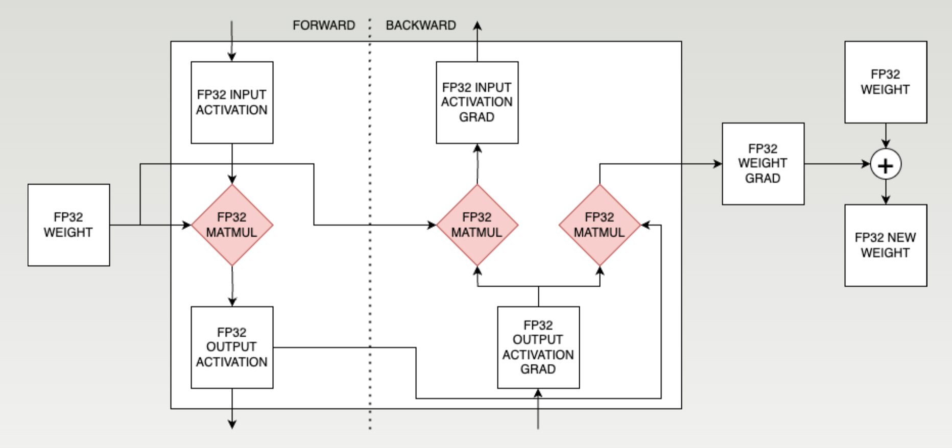
Each training step ultimately takes in the weights, does a bunch of matmuls with various data, and produces a new weight.

FP8 training is more complex. Below is a slightly simplified version of Nvidia’s FP8 training recipe.

Some notable features of this recipe

• Every matmul is FP8 x FP8 and accumulates into FP32 (it’s actually lower precision, but Nvidia tells everyone it is FP32), then is quantized to FP8 for the next layer. Accumulation must be in higher precision than FP8, because it involves tens of thousands of sequential small updates to the same large accumulator – so a lot of precision is needed for each small update to not round down to zero.

• Every FP8 weight tensor comes with a scale factor. Since each layer can have a dramatically different range, it is critical to scale each tensor to fit the range of the layer.

• The weight update (outside of the main box) is very sensitive to precision and generally has remain in a higher precision (generally FP32). This again comes down to a mismatch of magnitudes – the weight update is tiny compared to the weight, so again precision is needed for the update to not round down to zero.

Finally, one big difference with training versus inference is that gradients have much more extreme outliers, and this matters a lot. It’s possible to quantize the activation gradient (e.g. SwitchBack, AQT) to INT8, but the weight gradient has thus far resisted such efforts and must remain in FP16 or FP8 (1,5,2).

While quantization remains an extremely dynamic field as the HuggingFace model quantizers and hardware vendors alike strive for fewer bits, better accuracy, and energy efficiency. It’s far more subtle than just a number of bits though – there’s substantial complexity and a mix of all sorts of different formats in the hardware, all of which can be optimized.

We’ll need a lot more of this in coming years to keep up with Huang’s Law, and the hardware vendors aren’t keeping silent.

Get 20% off a group subscription

Nvidia, AMD, Intel, Google, Microsoft, Meta, Arm, Qualcomm, MatX and Lemurian Labs are targeting differening avenues of scaling, so lets break it down what they are doing.

Facebook Comments Box