Đào tạo đa trung tâm dữ liệu: Kế hoạch đầy tham vọng của OpenAI nhằm đánh bại cơ sở hạ tầng của Google
Buildouts of AI infrastructure are insatiable due to the continued improvements from fueling the scaling laws. The leading frontier AI model training clusters have scaled to 100,000 GPUs this year, with 300,000+ GPUs clusters in the works for 2025. Given many physical constraints including construction timelines, permitting, regulations, and power availability, the traditional method of synchronous training of a large model at a single datacenter site are reaching a breaking point.
Google, OpenAI, and Anthropic are already executing plans to expand their large model training from one site to multiple datacenter campuses. Google owns the most advanced computing systems in the world today and has pioneered the large-scale use of many critical technologies that are only just now being adopted by others such as their rack-scale liquid cooled architectures and multi-datacenter training.
Gemini 1 Ultra was trained across multiple datacenters. Despite having more FLOPS available to them, their existing models lag behind OpenAI and Anthropic because they are still catching up in terms of synthetic data, RL, and model architecture, but the impending release of Gemini 2 will change this. Furthermore, in 2025, Google will have the ability to conduct Gigawatt-scale training runs across multiple campuses, but surprisingly Google’s long-term plans aren’t nearly as aggressive as OpenAI and Microsoft.
Most firms are only just being introduced to high density liquid cooled AI chips with Nvidia’s GB200 architecture, set to ramp to millions of units next year. Google on the other hand has already deployed millions of liquid cooled TPUs accounting for more than one Gigawatt (GW) of liquid cooled AI chip capacity. The stark difference between Google’s infrastructure and their competitors is clear to the naked eye.
The AI Training campus shown above already has a power capacity close to 300MW and will ramp up to 500MW next year. In addition to their sheer size, these facilities are also very energy efficient. We can see below the large cooling towers and centralized facility water system with water pipes connecting three buildings and able to reject close to 200MW of heat. This system allows Google to run most of the year without using chillers, enabling a 1.1 PUE (Power Usage Effectiveness) in 2023, as per the latest environmental report.
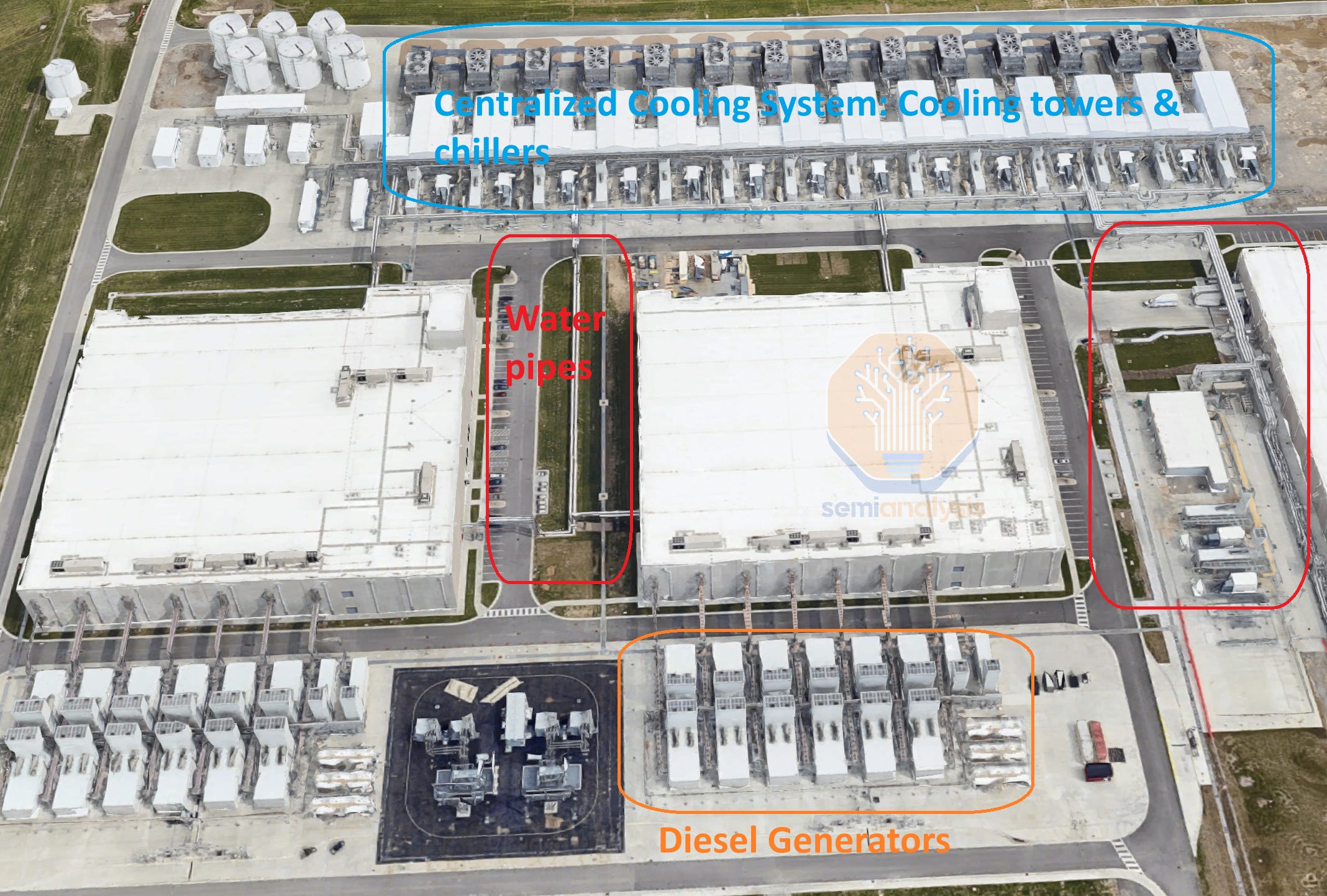
While the picture above only shows the facility water system, water is also delivered to the rack via a Direct-to-Chip system, with a Liquid-to-Liquid heat exchanger transferring heat from the racks to the central facility water system. This very energy-efficient system is similar to the L2L deployments of Nvidia GB200 – described in detail in our GB200 deep dive.
On the other hand, Microsoft’s largest training cluster today, shown below, does not support liquid cooling and has about 35% lower IT capacity per building, despite a roughly similar building GFA (Gross Floor Area). Published data reveals a PUE of 1.223, but PUE calculation is advantageous to air-cooled systems as Fan Power inside the servers are not properly accounted for – that’s 15%+ of server power for an air-cooled H100 server, vs <5% for a liquid DLC-cooled server. Therefore, for each watt delivered to the chips, Microsoft requires an extra ~45%+ power for server fan power, facility cooling and other non-IT load, while Google is closer to ~15% extra load per watt of IT power. Stack on the TPU’s higher efficiency, and the picture is murky.
In addition, to achieve decent energy efficiency in the desert (Arizona), Microsoft requires a lot of water – showing a 2.24 Water Usage Effectiveness ratio (L/kWh), way above the group average of 0.49 and Google’s average slightly above 1. This elevated water usage has garnered negative media attention, and they have been required to switch to air-cooled chillers for their upcoming datacenters in that campus, which will reduce water usage per building but further increase PUE, widening the energy efficiency gap with Google. In a future report, we’ll explore in much more detail how datacenters work and typical hyperscaler designs.
Therefore, based on existing Datacenter reference designs, Google has a much more efficient infrastructure and can build MWs much faster, given that each building has a >50% higher capacity and requires contracting less utility power per IT load.
Google always had a unique way of building infrastructure. While their individual datacenter design is more advanced than Microsoft, Amazon, and Meta’s today, that doesn’t capture the full picture of their infrastructure advantage. Google has also been building large-scale campuses for more than a decade. Google’s Council Bluffs Iowa site, shown below is a great illustration, with close to 300MW of IT capacity on the western portion despite being numerous years old. While significant capacity is allocated to traditional workloads, we believe that the building at the bottom hosts a vast number of TPU. The eastern expansion with their newest datacenter design will further increase the AI training capacity.
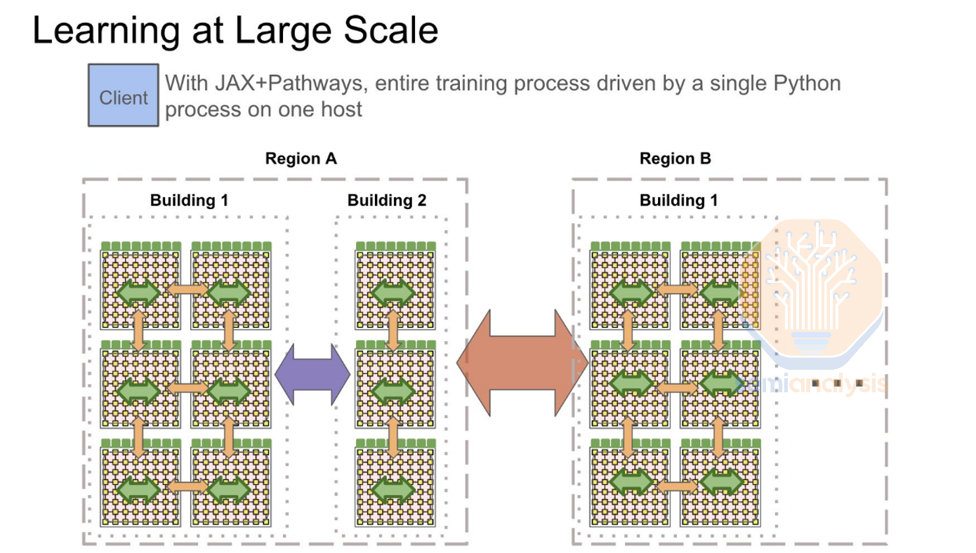
Google’s largest AI datacenters are also in close proximity to each other. Google has 2 primary multi-datacenter regions, in Ohio and in Iowa/Nebraska. Today, the area around Council Bluffs is actively being expanded to more than twice the existing capacity. In addition to the campus above, Google also owns three other sites in the region which are all under construction and are all being upgraded with high bandwidth fiber networks.
There are three sites ~15 miles from each other, (Council Bluffs, Omaha, and Papillon Iowa), and another site ~50 miles away in Lincoln Nebraska. The Papillion campus shown below adds >250MW of capacity to Google’s operations around Omaha and Council Bluffs, which combined with the above totals north of 500MW of capacity in 2023, of which a large portion is allocated to TPUs.
The other two sites are not as large yet but are ramping up fast: combining all four campuses will form a GW-scale AI training cluster by 2026. The Lincoln datacenter that is ~50 miles away will be Google’s largest individual site.
And Google’s massive TPU footprint does not stop here. Another upcoming GW-scale cluster is located around Columbus, Ohio – the region is following a similar leitmotif, with three campuses being developed and summing up to 1 Gigawatt by the end of 2025!
The New Albany cluster, shown below, is set to become one of Google’s largest and is already hosting TPU v4, v5, v6.
The concentrated regions of Google Ohio and Google Iowa/Nebraska could also be further interconnected to deliver multiple gigawatts of power for training a single model. We have precisely detailed quarterly historical and forecasted power data of over 5,000 datacenters in the Datacenter Model. This includes status of cluster buildouts for AI labs, hyperscalers, neoclouds, and enterprise. More on the software stack and methods for multi-datacenter training later in this report.
Microsoft and OpenAI are well aware of their disadvantages on infrastructure for the near term and have embarked on an incredibly ambitious infrastructure outbuild Google. They are trying to beat Google in their own game of water-cooled multi-datacenter training clusters.
Microsoft and OpenAI are constructing ultra-dense liquid-cooled datacenter campuses approaching the Gigawatt-scale and also working with firms such as Oracle, Crusoe, CoreWeave, QTS, Compass, and more to help them achieve larger total AI training and inference capacity than Google.
Some of these campuses, once constructed, will be larger than any individual Google campus today. In fact, Microsoft’s campus in Wisconsin will be larger than all of Google’s Ohio sites combined but building it out will take some time.
Even more ambitious is OpenAI and Microsoft’s plan to interconnect various ultra large campuses together, and run a giant distributed training runs across the country. Microsoft and OpenAI will be first to a multi-GW computing system. Along with their supply chain partners they are deep into the most ambitious infrastructure buildout ever.
This report will detail Microsoft and OpenAI’s infrastructure buildout closer to the end. Before that it will first cover multi-campus synchronous and asynchronous training methods, stragglers, fault tolerance, silent data corruption, and various challenges associated with multi-datacenter training.
Then we will explain how datacenter interconnect as well as metro and long-haul connectivity between datacenters is enabled by fiber optic telecom networks, both technology and equipment.
Finally, we will explore the telecom supply chain and discuss key beneficiaries for this next leg of the AI infrastructure buildouts including which firms we believe are the most levered to this.
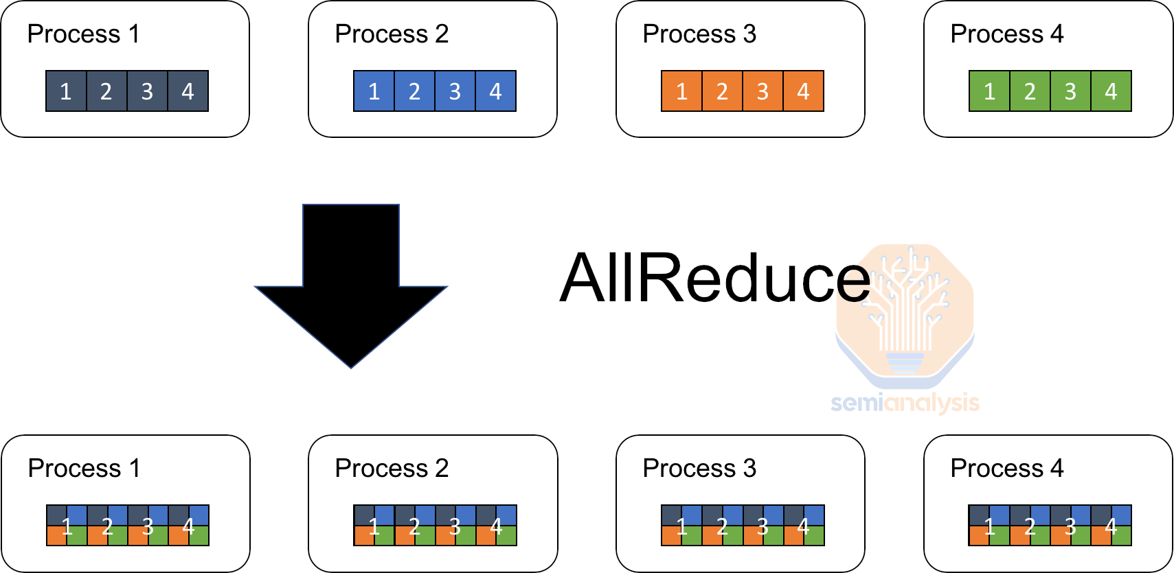
Before jumping into the Microsoft OpenAI infrastructure buildouts, first a primer on distributed training. Large language models (LLMs) are primarily trained synchronously. Training data is typically partitioned into several smaller mini-batches, each processed by a separate data replica of the model running on different sets of GPUs. After processing a mini-batch, each replica calculates the gradients, then all replicas must synchronize at the end of each mini-batch processing.
This synchronization involves aggregating the gradients from all replicas, typically through a collective communication operation like an all-reduce. Once the gradients are aggregated, they are averaged and used to update the model’s parameters in unison. This ensures that all data replicas maintain an identical set of parameters, allowing the model to converge in a stable manner. The lock-step nature of this process, where all devices wait for each other to complete before moving to the next step, ensures that no device gets too far ahead or behind in terms of the model’s state.
While synchronous gradient descent offers stable convergence, it also introduces significant challenges, particularly in terms of increased communication overhead as you scale above 100k+ chips within a single training job. The synchronous nature also means that you have strict latency requirements and must have a big pipe connecting all the chips since data exchanges happen in giant bursts.
As you try to use GPUs from multiple regions towards the same training workload, the latency between them increases. Even at the speed of light in fiber at 208,188 km/s, the round-trip time (RTT) from US east coast to US west coast is 43.2 milliseconds (ms). In addition, various telecom equipment would impose additional latency. That is a significant amount of latency and would be hard to overcome for standard synchronous training.
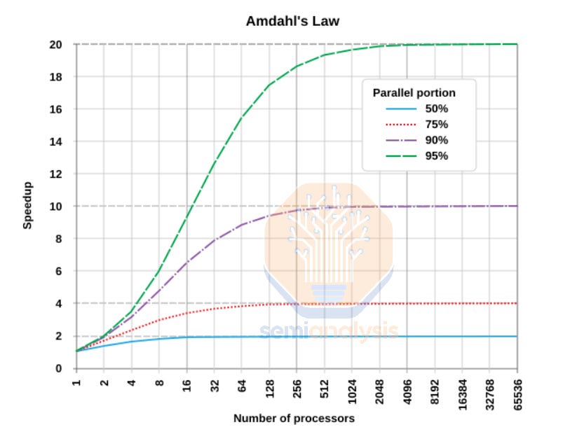
According to Amdahl’s Law, the speedup from adding more chips to a workload has diminishing returns when there is a lot of synchronous activity. As you add more chips, and the portion of the program’s runtime that needs synchronization (i.e. corresponding to the proportion of the calculation that remains serial and cannot be parallelized) remains the same, you will reach a theoretical limit where even doubling the number of GPUs will not get you more than a 1% increase in overall throughput.
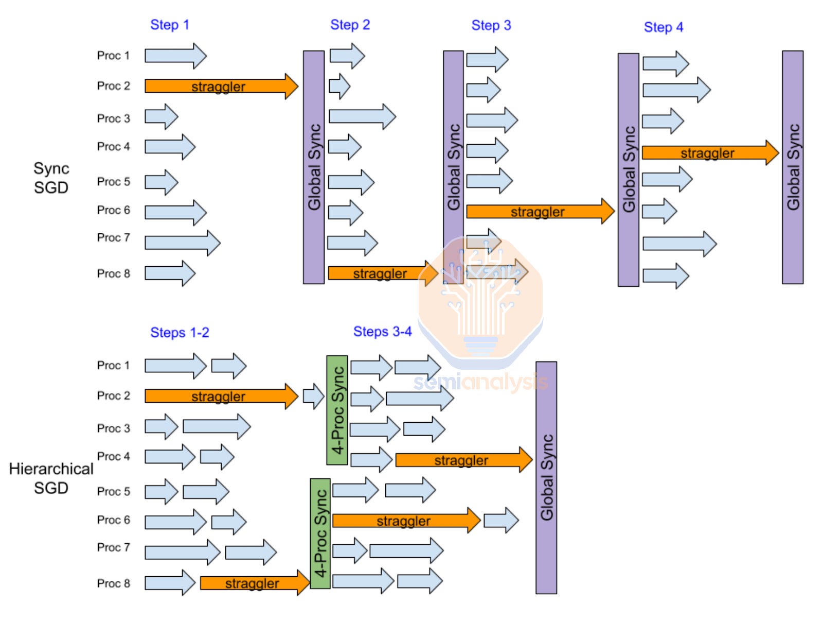
In addition to the theoretical limits of scaling more GPUs towards a single workload described by Amdahl’s Law, there are also the practical challenges of Synchronous Gradient Descent such as stragglers. When just one chip is slower by 10%, it causes the entire training run to be slower by 10%. For example, in the diagram below, from step 7,500 to step 19,000, ByteDance saw their MFU slowly decrease as, one by one, more chips within the workload became slightly slower and the entire workload became straggler-bound.
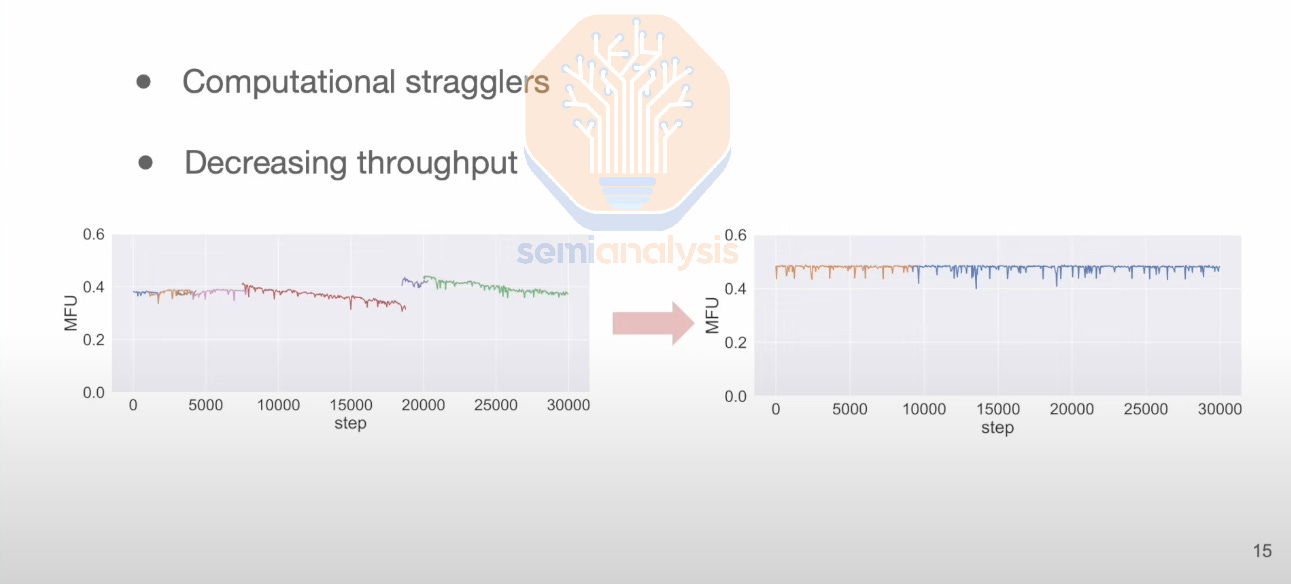
After identifying and removing the stragglers, they restarted the training workload from a checkpoint, increasing MFU back to a normal level. As you can see, MFU went from 40% to 30%, a 25% percentage decrease. When you have 1 million GPUs, a 25% decrease in MFU is the equivalent of having 250k GPUs running idle at any given time, an equivalent cost of over $10B in IT capex alone.
Fault Tolerant training is an essential part of all distributed systems. When millions of computing, memory, and storage elements are working, there will always be failures or even just silicon lottery in terms of performance differences between various “identical” systems. Systems are designed to deal with this. Counterintuitively in the world’s largest computing problem, machine learning training, the exact opposite approach is used.
All chips must work perfectly because if even one GPU fails out of 100k GPUs, this GPU will cause all 100k GPU to restart from checkpoint, leading to an insane amount of GPU idle time. With fault tolerant training, when a single GPU fails, only a few other GPUs will be affected, the vast majority continuing to run normally without having to restart from a model weights checkpoint. Open models such as LLAMA 3.1 have had significant cost and time burned due to this.
Nvidia’s InfiniBand networking also has this same potentially flawed principle in that every packet must be delivered in the exact same order. Any variation or failure leads to a retransmit of data. As mentioned in the 100,000 GPU cluster report, failures from networking alone measure in minutes not hours.

The main open-source library that implements fault tolerant training is called TorchX (previously called TorchElastic), but it has the significant drawbacks of not covering the long tail of failure cases and not supporting 3D parallelism. This has led to basically every single large AI lab implementing their own approach to fault tolerant training systems.
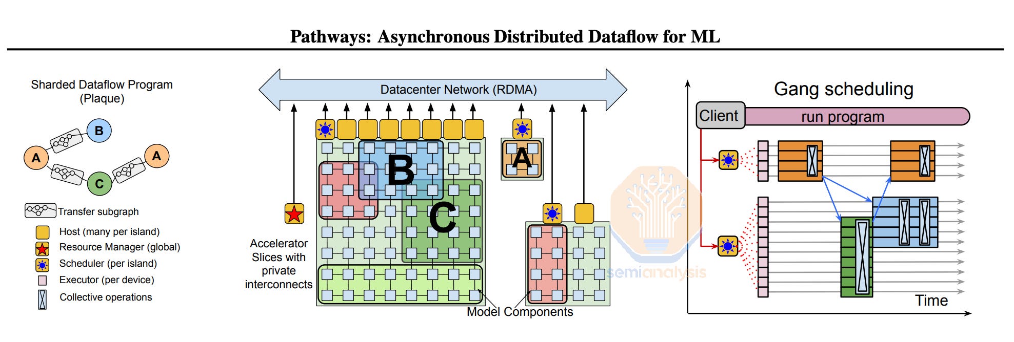
As expected, Google, the leader in fault tolerance infrastructure, has the best implementation of fault tolerant training through Borg and Pathways. These libraries cover of the greatest number of corner cases and are part of a tight vertical integration: Google is designing their own training chips, building their own servers, writing their own infra code, and doing model training too. This is similar to building cars where the more vertically integrated you are, the more quickly you can deal with root causing manufacturing issues and solving them. Google’s Pathways system from a few years ago is a testament to their prowess, which we will describe later in this report.
In general, fault tolerance is one of the most important aspects to address in scaling clusters of 100k+ GPUs towards a single workload. Nvidia is way behind Google on reliability of their AI systems, which is why fault tolerance is repeatedly mentioned in NVIDIA’s job descriptions…
Tolerance infrastructure in CPU-land is generally a solved problem. For example, Google’s in house database, called Spanner, runs all of Google’s production services including Youtube, Gmail, and Stadia (RIP) among others, and is able to distribute and scale across the globe while being fault tolerant with respect to storage server and NVMe disk failures. Hundreds of NVMe disks fail per hour in Google datacenters, yet to the end customer and internally, the performance and usability of Spanner stays the same.
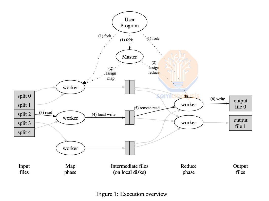
Another example of fault tolerance in traditional CPU workloads on Large Cluster is MapReduce. MapReduce is a style of modelling where users can “map” a data sample by processing it and “reduce” multiple data samples into an aggregated value. For example, counting how many letter “W’s” are in an essay is a great theoretical workload for map-reduce: map each word, the map will output how many letter “W”s are in each data sample, and “reduce” will aggregate the number of “W”s from all the samples. MapReduce can implement Fault Tolerance by detecting which CPUs workers are broken and re-execute failed map and reduce tasks on another CPU worker node.
A significant portion of fault tolerance research and systems in CPU land have been developed by Jeff Dean, Sanjay Ghemawat, and the many other world class distributed systems experts at Google. This expertise in creating robust, reliable systems will be one of Google’s competitive advantages as ML training gets larger and requires better fault tolerance ML training systems.
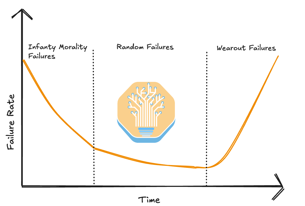
Generally, GPU failure follows a bathtub shape curve where most of the failures happen towards the beginning (i.e. infant mortality failures) and near the end of a cluster’s lifespan. This is why cluster-wide burn-in is extremely important. Unfortunately, due to their goal of trying to squeeze the most money out of a cluster’s lifespan, a significant proportion of AI Neoclouds do not properly burn in their cluster, leading to an extremely poor end user experience.
In contrast, at hyperscalers and big AI labs, most clusters will be burnt in at both high temperatures and rapidly fluctuating temperatures for a significant amount of time to ensure that all the infant mortality failures are past and have shifted into the random failure phrase. Adequate burn in time must be balanced against using too much of the useful life of GPUs and transceivers once they are past early issues.
The wear out failures phase is when components fail at end of life due to fatigue. Often from rapid fluctuation between medium and high temperatures over a 24/7 usage period. Transceivers in particular suffer from high wear and tear due to severe thermal cycling.
In CPU land, it is common to migrate Virtual Machines (VMs) between physical hosts when the physical host hosting the VM is showing signs of an increased error rate. Hyperscalers have even figured out how to live migration VMs between physical hosts without the user end even noticing that it has been migrated. This is generally done by copying pages of memory in the background and then, when the user’s application slows down for a split second, the VM will be switched rapidly onto the second, normally functioning physical host.
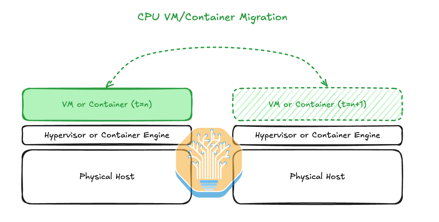
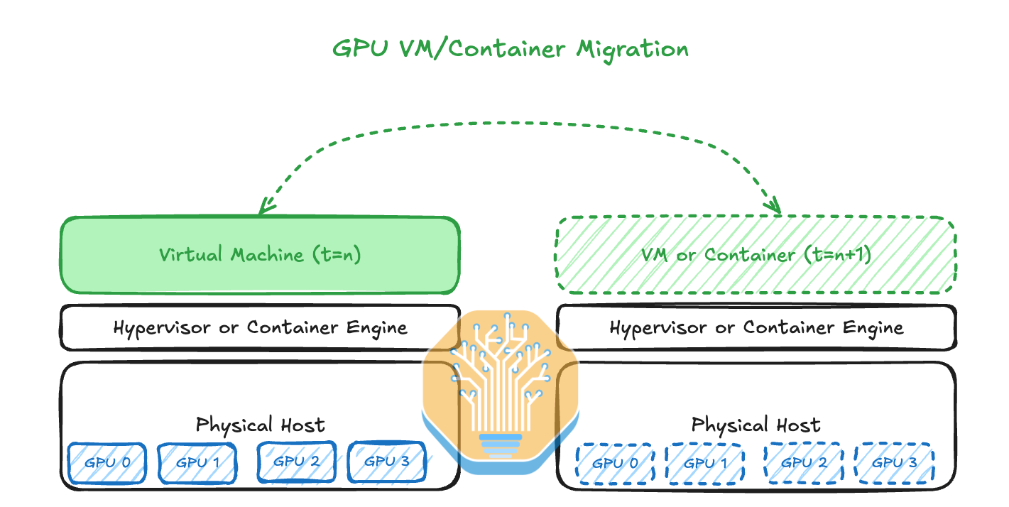
There is a mainstream Linux software package called CRIU (Checkpoint/Restore In Userspace) that is used in major container engines such as Docker, Podman and LXD. CRIU enables migrating containers and applications between physical hosts and even freezes and checkpoints the whole process state to a storage disk. For a long time, CRIU was only available on CPUs and AMD GPUs as Nvidia refused to implement it until this year.
With GPU CRIU checkpointing now available on Nvidia GPUs from the beginning of 2024, one can now migrate the CPU process state, memory content and GPU processes from one physical host to another in a far more streamlined manner.
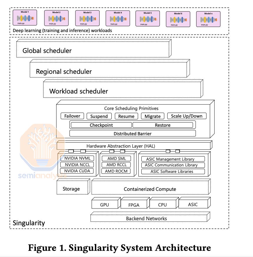
In Microsoft’s Singularity Cluster Manager paper the authors described their method of using CRIU for transparent migration of GPU VMs. Singularity is also designed from the ground up to allow for global style scheduling and management of GPU workloads. This system has been used for Phi-3 training (1024 H100s) and many other models. This was Microsoft playing catchup with Google’s vertically integrated Borg cluster manager.
Unfortunately, due to the importance of fault tolerant training, publishing of methods has effectively stopped. When OpenAI and others tell the hardware industry about these issues, they are very vague and high level so as to not reveal any of their distributed systems tricks. To be clear, these techniques are more important than model architecture as both can be thought of as compute efficiency.
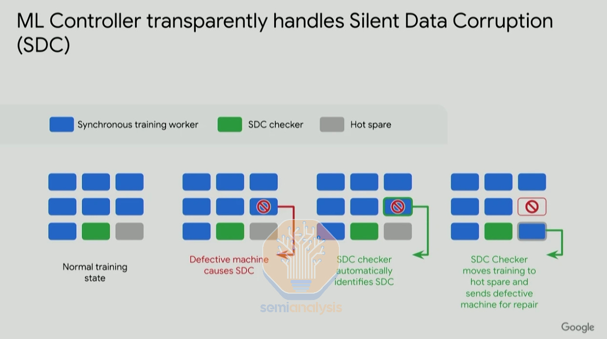
Another common issue is Silent Data Corruption (SDC), which leads computers to inadvertently cause silent errors within the results processed, without any alert to users or administrators. This is a very difficult problem to solve as silent literally means the error is unnoticeable. These silent errors can be trivial in many cases, but they can also cause outputs to be distorted into NaNs (“Not A Number”) or the output gradient to be extremely large. As shown in the gradient norm graph below from Google’s Jeff Dean, some SDCs can be easily identified visually when charted as gradient norm spikes up, but there are other SDCs undetectable by this method.
There are also gradient norm spikes that are not caused by hardware SDCs and are in fact caused by a big batch of data or hyperparameters like learning rate and initialization schemes not being properly tuned. All companies running GPU clusters regularly experience SDCs, but it is the generally small and medium Neoclouds that are unable to quickly identify and fix them due to limited resources.
For Nvidia GPUs, there is a tool called DCGMI Diagnostics that helps diagnose GPU errors such as SDCs. It helps catch a good chunk of common SDCs but unfortunately misses a lot of corner cases that result in numerical errors and performance issues.
Something we experienced in our own testing of H100s from various Neoclouds was that DCGMI diagnostic level 4 was passing, but NVSwitch’s Arithmetic Logic Unit (ALU) was not working properly, leading to performance issues and wrong all-reduce results when utilizing the NVLS NCCL algorithm. We will dive much deeper into our benchmarking findings in an upcoming NCCL/RCCL collective communication article.
Google’s Pathways, in contrast, excels at identifying and resolving SDCs. Due to the vertical integration of Google’s infrastructure and training stack, they are able to easily identify SDC checks as epilogue and prologue before starting their massive training workloads.
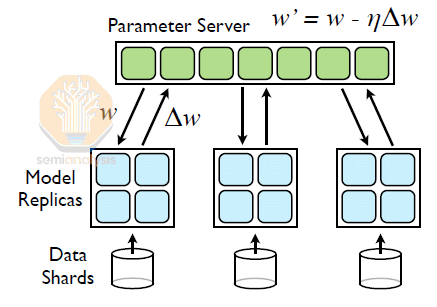
Asynchronous training used to be a widespread training technique. In 2012, Jeff Dean, the famous 100x engineer from Google Brain, published a paper called Distbelief where he describes both asynchronous (“Async”) and synchronous (“Sync”) gradient descent techniques for training deep learning models on a cluster of thousands of CPU cores. The system introduced a global “parameters server” and was widely used in production to train Google’s autocompletion, search and ad models.
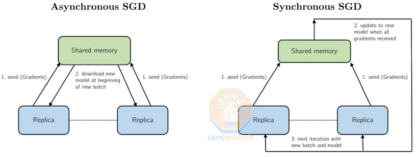
This parameter server style training worked very well for models at the time. However, due to convergence challenges with newer model architectures, everyone just simplified their training by moving back to full synchronous gradient descent. All current and former frontier-class models such as GPT-4, Claude, Gemini, and Grok are all using synchronous gradient descent. But to continue scaling the number of GPUs used in a training run, we believe that there is currently a shift back to asynchronous gradient descent.
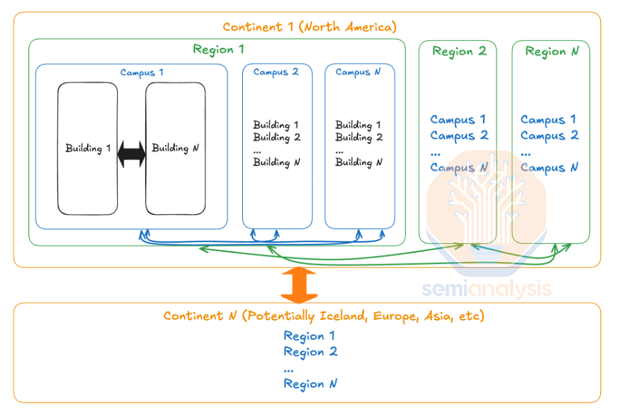
In Amdahl’s Law, one way of getting around the diminishing returns when adding more chips is to decrease the number of global syncs you need between programs and allow more of the workload to operate (semi)-independently as a percentage of wall time clock. As you can imagine, this maps well to multi-campus, multi-region and cross-continent training as there is a hierarchy of latency and bandwidth between various GPUs.
Between buildings within a campus, which are very close together (less than 1km), you have very low latency and very high bandwidth and thus are able to synchronize more often. In contrast, when you are within a region (less than 100km), you may have a lot of bandwidth, but the latency is higher, and you would want to synchronize less often. Furthermore, it is acceptable to have different numbers of GPUs between each campus as it is quite easy to load balance between them. For instance, if Campus A has 100k GPUs and Campus B has only 75k GPUs, then Campus B’s batch size would probably be about 75% of Campus A’s batch size, then when doing the syncs, you would take a weighted average across the different campuses.
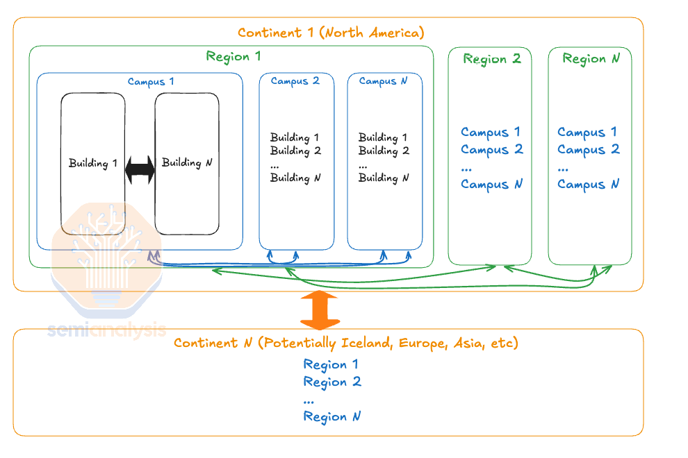
This principle can be applied between multiple regions and cross-continents where latency is higher, and as such, you should sync even less. Effectively – there is a hierarchy of sync’ing.
To use an analogy this is akin to how you tend to see friends that are closer to you in terms of distance more often than your friends in other cities on the same coast, and you tend to see your friends on the same coast more often than your friends in cities on other continents.
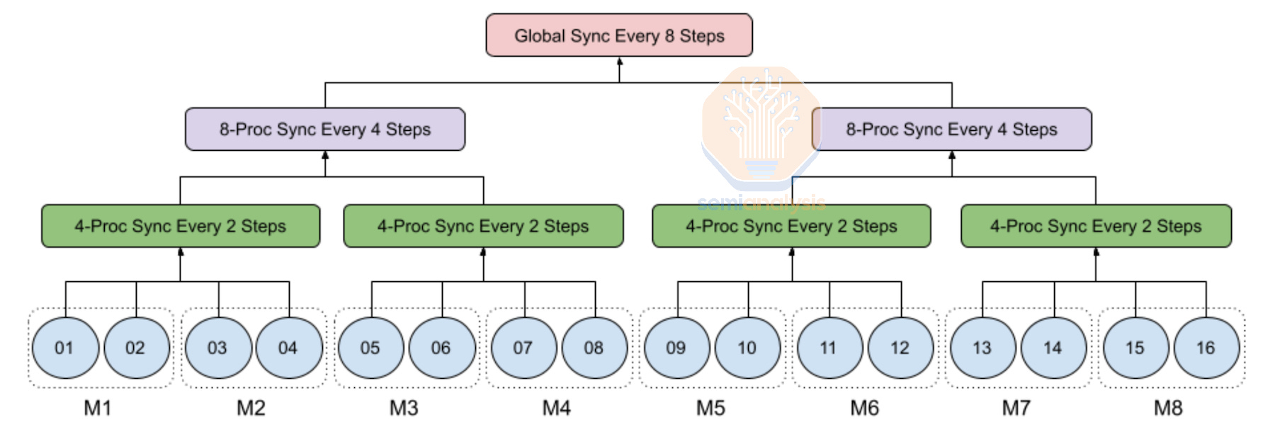
Moreover, another benefit of hierarchy synchronous gradient descent (SGD) is that it helps mitigate stragglers as most stragglers usually appear during a couple of steps but then return to their normal performance, so the fewer syncs there are, the fewer opportunities there are for stragglers to disrupt the sync process during their episodes of abnormal performance. Since there is no global sync at every iteration, the effects of stragglers are less prominent. Hierarchal SGD is a very common innovation for multi-datacenter training in the near term.
Another promising method is to revisit the use of asynchronous parameter servers as discussed in Jeff Dean’s 2012 DistBelief paper. Each replica of the model processes its own batch of the tokens and every couple of steps, each replica will exchange data with the parameter servers and update the global weights. This is like git version control where every programmer works on their own task for a couple of days before merging it into the master (now called main) branch. A naïve implementation of this approach would likely create convergence issues, but OpenAI will be able to solve update issues in exchanging data from the local model replica into the parameter using various optimizer innovations.
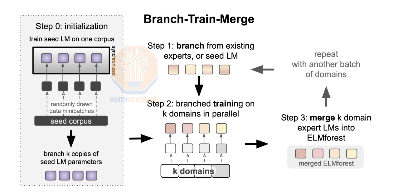
MetaAI’s Branch-Train-Merge paper describes a similar idea where you branch from an existing LLM (master branch) then train on the subset of the dataset before merging it back into the master branch. We believe that learnings from this approach will be incorporated into multi-campus training techniques that companies such as OpenAI will end up using. The main challenge with Branch-Train-Merge and other similar approaches is that merging is not a solved problem for modern LLMs when it comes to classes of models such as GPT3 175B or GPT4 1.8T. More engineering resources will need to be poured into managing merges and updating the master branch in order to maintain convergence.
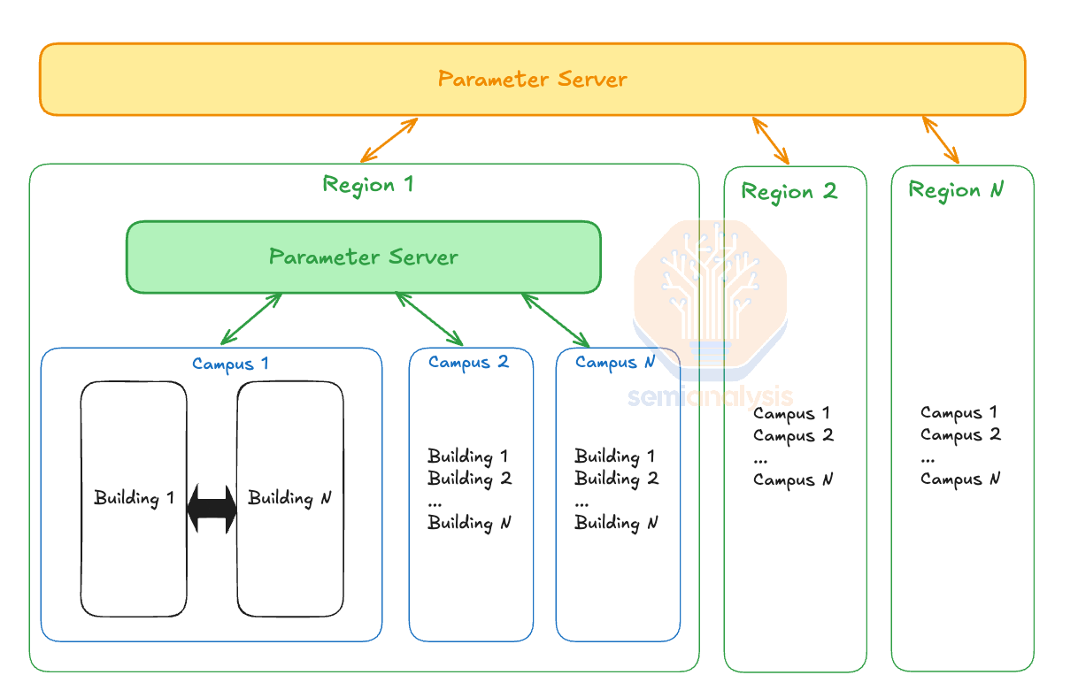
To extend this into a hierarchy approach, we need to also have tiers of parameter servers where data is exchanged between model replicas and the closest parameters servers and also between parameters servers. At the lowest level, individual model replicas communicate with their closest parameter servers, performing updates more frequently to ensure faster convergence and synchronization within local groups.
These local parameter servers will be grouped into higher tiers where each tier aggregates and refines the updates from the lower levels before propagating them upwards. Due to the immense number of GPUs involved, parameter servers will probably need to hold the master weights in FP32. This is similar to how Nvidia’s recommended FP8 training server holds the master weights in FP32 so that it doesn’t overflow from many GPUs accumulating. However, before doing the matrix multiply the training servers will downcast to FP8 for efficiency. We believe that this recipe will still hold true where the master weights in the parameter server will be FP32 but the actual calculations will be performed in FP8 or even lower such as MX6.
To achieve multi-campus training, Google currently uses a powerful sharder called MegaScaler that is able to partition over multiple pods within a campus and multiple campuses within a region using synchronous training with Pathways. MegaScaler has provided Google a strong advantage in stability and reliability when scaling up the amount of chips contributing towards a single training workload.
This could be a crutch for them as the industry moves back towards asynchronous training. MegaScaler is built atop the principle of synchronous-style training where each data replica communicates with all other data replicas to exchange data. It may be difficult for them to add asynchronous training to MegaScaler and may require a massive refactor or even starting a new greenfield project. Although Pathways is built with asynchronous dataflow in mind, in practice, all current production use cases of Pathways are fully synchronous SGD style training. With that said, Google obviously has the capabilities to redo this software stack.
There are two main limitations when networking datacenters across regions: bandwidth and latency. We generally believe that longer term the limiting factor will be the latency due to speed of light in glass, not bandwidth. This is due to the cost of laying down fiber cables between campus and between regions is mostly the cost of permitting and trenching and not the fiber cable itself. Thus laying 1000 fiber pairs between say Phoenix and Dallas will only be slightly higher cost than laying down 200 fiber pairs. With that said, the industry operates in a regulatory framework and timescales in which fiber pairs cannot be laid in an instant, therefore strategies for reducing bandwidth are still very critical.
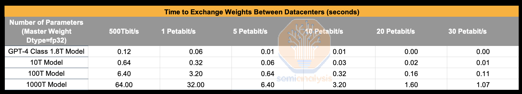
We believe the models that will be trained on this multi-campus, multi-region training cluster will be on the order of magnitude of 100T+. Between AZs within a region, we believe that growing to around 5Pbit/s between campus sites within a region is a reasonable assumption of what they can scale to within the near future, while 1Pbit/s is a reasonable amount of bandwidth between regions. If the cross-datacenter bandwidth is that truly that high, exchanging weights between campus sites is not a major bottleneck for training as it only takes 0.64 seconds at line rate. When exchanging 400TeraBytes (4Bytes = param) of weights, only taking 0.64 seconds is very good considering how much time it will take for every couple of compute steps.
While Nvidia offers an InfiniBand fabric networking switch called MetroX within 40kms, no AI lab uses it, only a couple of non-AI HPC clusters that span multiple campuses within 10km. Furthermore, it only has 2x100Gbps per chassis versus the quite mature ecosystem of metro <40km ethernet solutions. As such even Microsoft, who uses InfiniBand heavily, uses Ethernet between datacenters.
Networks within datacenters (i.e. Datacom) today typically focus on delivering speeds of up to 400Gbps per end device (i.e. per GPU) over a fiber link, with the transition to 800Gbps for AI usage to be well underway next year driven by Nvidia’s transition to Connect-X8 Network Interface Cards (NICs).
In contrast, telecom networks take communications needs for multiple devices and servers within one facility, and aggregate this onto a smaller number of fibers that run at far greater speeds. While datacom transceivers running 800 Gbps will often utilize only up to 100 Gbps per fiber pair (DR8), requiring multiple separate fiber pairs, telecom applications already fit in excess of 20-40Tbps on just one single-mode fiber pair for submarine cables and many terrestrial and metro deployments.
Greater bandwidth is achieved by a combination of
-
Higher order modulation schemes, delivering more bits per symbol on a given wavelength.
-
Dense Wave Division Multiplexing (DWDM), which combines multiple wavelengths of light onto a single fiber.
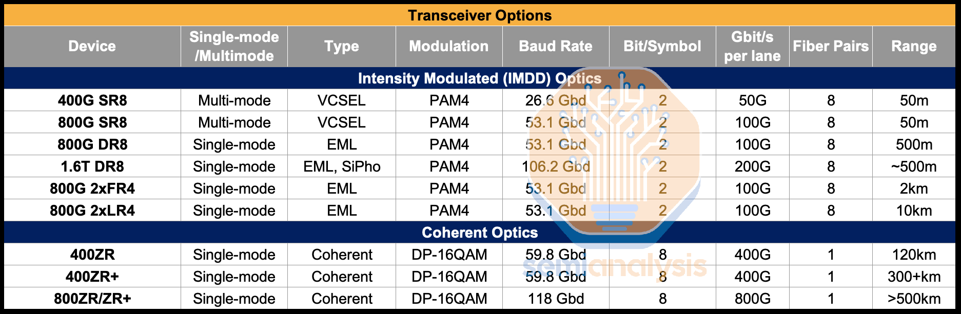
On the modulation front, Datacom typically uses VCSEL and EML based transceivers that are capable of PAM4 modulation, an intensity modulation scheme (i.e. Intensity Modulated Direct Detection – IMDD optics) which is achieved by using four different levels to signal, encoding two bits of data per symbol.
Higher speeds are achieved by either increasing the rate at which symbols are sent (measured in Gigabaud or Gbd) or increasing the number of bits per symbol. For example, a 400G SR8 transceiver could transmit symbols at 26.6 Gbd and use PAM4 to achieve 2 bits per symbol, for a total of 50 Gbps per fiber pair. Combine 8 fiber pairs into one connector and that reaches 400 Gbps overall. Reaching 800Gbps overall could be achieved by increasing the symbol rate to 53.1 Gbd while still using PAM4 across 8 lanes. However, doubling the symbol rate is often a more difficult challenge than using higher order modulation schemes.
16-Quadrature Amplitude Modulation (or 16-QAM) is one such scheme that is widely used in ZR/ZR+ optics and telecom applications. It works by not only encoding four different amplitudes of signal waves, but also using two separate carrier waves that can each have four different amplitudes and are out of phase with each other by 90 degrees, for a total of 16 different possible symbols, delivering 4 bits per symbol. This is further extended by implementing dual polarization, which utilizes another set of carrier waves, with one set of carrier waves on a horizontal polarization state and the other on a vertical polarization state, for 256 possible symbols, achieving 8 bits. Most 400ZR/ZR+ and 800ZR/ZR+ transceivers only support up to DP-16QAM, but dedicated telecom systems (with a larger form factor) running on good quality fiber can support up to DP-64QAM for 12 bits per symbol.
To implement modulation schemes using different phases, coherent optics (not to be confused with Coherent the company) are required. Light is considered coherent when the light waves emitted by the source are all in phase with one another – this is important in implementing phase-based modulation schemes because an inconsistent (non-coherent) light source would result in inconsistent interference, making recovery of a phase modulated signal impossible.
Coherent optics require the use of a coherent Digital Signal Processor (DSP) capable of processing higher order modulation schemes, as well as a tunable laser and a modulator, though in the case of 400ZR, silicon photonics are often used to achieve lower cost. Note the tunable laser is very expensive as well and as such, there are attempts to use cheaper O-band lasers in coherent-lite.
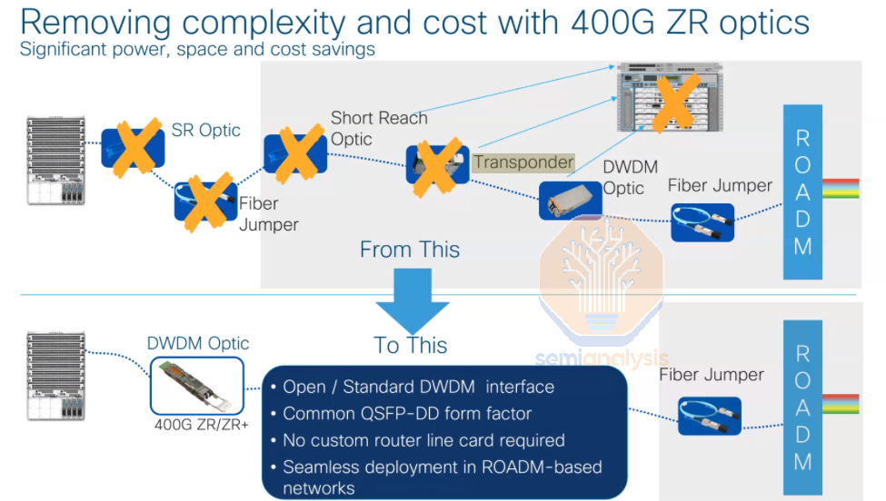
ZR/ZR+ optics are an increasingly popular transceiver type that use coherent optics and are designed specifically for datacenter interconnect, delivering much greater bandwidth per fiber pair and achieving a far greater reach of 120km to 500km. They also typically come in an OSFP or QSFP=DD form factor – the same as is commonly used for datacom applications – meaning they can plug directly into the same networking switches used in datacom.
Traditional telecom systems can be used for datacenter interconnect, but this requires a much more complicated chain of telecom equipment occupying more physical space in the datacenter compared to ZR/ZR+ pluggables, which can plug directly into a networking port on either end, sidestepping several telecom devices.
Higher order modulation schemes enable more bandwidth per fiber pair, 8x more in the case of DP-16QAM, as compared to Intensity Modulated Direct Detection (IMDD) transceivers using PAM4. Long reach still has fiber limitations though, so Dense Wave Division Multiplexing (DWDM) can also be used to enable even more bandwidth per fiber pair. DWDM works by combining multiple wavelengths of light into one fiber pair. In the below example, 76 wavelengths on the C band (1530nm to 1565nm) and 76 wavelengths on the L band (1565nm to 1625nm) are multiplexed together onto the same fiber.
If 800Gbps per wavelength can be deployed on this system – this could yield up to 121.6Tbps for a single fiber pair. Submarine cables will typically maximize the number of wavelengths used, while some deployments might use less than 16 wavelengths, though it is not unheard of to have deployments using 96 wavelengths, with current typical deployments targeting 20-60 Tbps per fiber pair.
Many deployments start by lighting up only a few wavelengths of light on the C-band and expand along with customer demand by lighting up more of the C-band and eventually the L-band, enabling existing fibers to be upgraded massively in speed over time.
Most US metros still have an abundance of fiber that can be lit up and harnessed, and the massive bandwidth required by AI datacenter interconnect is a perfect way to sweat this capacity. In submarine cables, consortiums often only deploy 8-12 pairs of fiber as deployment cost scales with number of fiber pairs due to physical cable and deployment. In terrestrial cables, most of the cost is in labor and equipment (and right of way in some urban areas) to dig up the trenches as opposed to the physical fiber, so companies tend to lay hundreds if not thousands of pairs when digging up terrestrial routes in metro areas.
Training across oceans will be significantly more difficult than training across land.
A typical fiber optics business case might assume a considerable number of fiber pairs left fallow for future demand. And it is not just metros, but generally any major road, transmission line, railway, or piece of infrastructure tends to have fiber optic cables running alongside – anyone building infrastructure will tend to deploy fiber alongside as a side business as it attracts minimal incremental cost if you’re going to have trenching crews on site anyways.
When it comes to hyperscaler telecom networks, the preference is to build their own networks as opposed to working with telecom providers, working directly with equipment vendors and construction companies for long haul, metro, and datacenter interconnect needs.
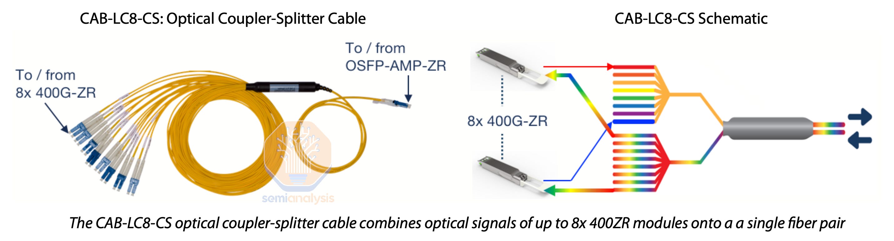
Datacenter interconnect, connecting two datacenters less than about 50km apart in a point-to-point network, is typically built by laying down thousands of fiber optic pairs. The hyperscaler can plug ZR transceivers into network switches inside each of the two distant datacenters, and either tune the transceivers to different wavelengths of light then combine up to 64 transceivers onto a single fiber pair using a passive multiplexer (i.e. a DWDM link), reaching up to 25.5 Tbps per fiber pair if using 400ZR, or simply plug each ZR transceiver into its own fiber pair.
More elaborate telecom systems also implementing DWDM can be used to multiplex many more ZR optics signals onto fewer number of fiber pairs and enable more than just a point-to-point network, but this would require a few racks of space for telecom equipment to house routers, ROADMs, and multiplexers/demultiplexers needed for DWDM.
Since most of the cost is in digging up the trench for the optics, most hyperscalers find it easier to deploy a lot more fiber pairs than needed, saving space within the data hall and avoiding a more complicated telecom deployment. They would typically only resort to deploying extensive telecom systems for short distances if they are deploying fiber in locations that have constraints in obtaining physical fiber capacity, which can be the case outside the United States, when hyperscalers might be forced onto as little as 2-4 fiber pairs in metros with scarce fiber availability.
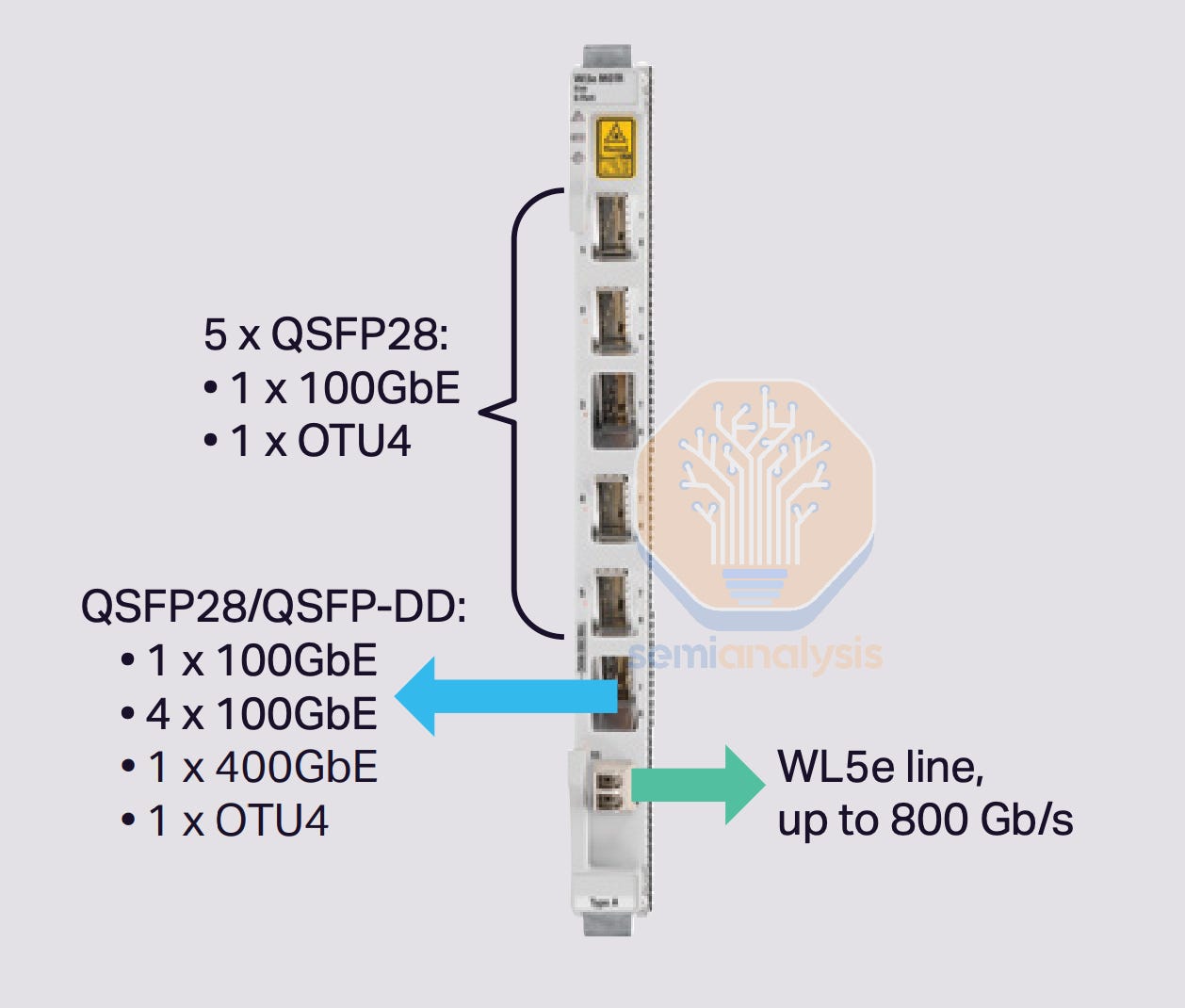
For long-haul networks however, hyperscalers will need to employ a full suite of telecom products that are very distinct from products used in datacom. A typical long-haul network will at least require a few basic systems: Transponders, DWDM Multiplexers/Demultiplexers, Routers, Amplifiers, Gain Equalizers, and Regenerator Sites, and in most but not all cases, ROADMs (Reconfigurable Optical Add/Drop Multiplexers) and WSSs (Wavelength Selective Switches).
A transponder provides a similar function to a transceiver in the telecom space but is much more expensive and operates at higher power levels. One side transmits/receives into the actual telecom network (line side), with the other offering many possible combinations of ports to connect to client devices (client side) within that location. For example, a transponder might offer 800Gbps on the line side, and 4 ports of 200Gbps optical or electric on the client side, but there are innumerable combinations of port capacities and electrical/optical that customers can choose from. The client side could connect to routers or switches within a datacenter, while the line side will connect to Multiplexers to combine many transponders’ signals using DWDM and potentially ROADMs to allow optical switching for network topologies more complicated than simple point-to-point connectivity.
DWDM works using a multiplexer and demultiplexer (mux/demux) that takes slightly different wavelengths of light signals from each transponder and combines it onto one fiber optic pair. Each transponder is tunable and can dial in specific wavelengths of light for the multiplexing onto that same fiber pair. When using a ROADM, transponders will typically connect to a colorless mux/demux, and from there to a Wavelength Selective Switch (WSS), allowing the ROADM to dynamically tune transponders to specific wavelengths in order to optimize for various network objectives.
Optical amplifiers are needed to combat the attenuation of light signals over long distances on fiber. Amplifiers are placed every 60-100km on the fiber route and can amplify the optical signal directly without having to convert the optical signal to an electrical signal. A gain equalizer is needed every after three amplifiers to ensure that different wavelengths of light traveling at different speeds are equalized to avoid errors. In some very long-haul deployments of thousands of kilometers, regeneration is needed, which involves taking the optical signal off into electronics, reshaping and retiming the signal, and retransmitting it using another set of transponders.
If the network connects more than two points together and has multiple stops where traffic is added or received at, then a ROADM (Reconfigurable Optical Add/Drop Multiplexer) is needed. This device can optically add or drop specific wavelengths of light at a given part of the network without having to offload any of the signals to an electrical form for any processing or routing. Wavelengths that are to be transmitted or received by a given location can be added or dropped from the main fiber network, while others that do not carry traffic to that location can travel through the ROADM unimpeded. ROADMs also have a control plane and it can actively discover and monitor the network state, understanding which channels on the fiber network are free, channel signal to noise ratio, reserved wavelengths, and as discussed above, can control transponders, tuning the line side to the appropriate wavelength.
These various components are typically combined together in a modular chassis that could look something like this:
Ciena, Nokia, Infinera and Cisco are a few major global suppliers of telecom systems and equipment, while Lumentum, Coherent, Fabrinet and Marvell provide various subsystems and active components to these major suppliers. Much of the strength for the component players so far has been seen in ZR/ZR+ optics for datacenter interconnect, but as hyperscalers and other operators have to get serious about training beyond adjacent data centers, they could potentially significantly hike their spending on much higher ASP telecom equipment and systems.
Demand for telecom equipment from non-cloud customers also appears to have troughed and could enter a recovery phase of the cycle soon – boosting the fortunes of various telecom suppliers.
Next, let’s discuss the ambitious multi-datacenter training plans of OpenAI and Microsoft as well as the winners in the telecom space for this massive buildout.
